ML Interview Q Series: Projecting LDA Centroids Below K-1 Dimensions Using Eigendecomposition

📚 Browse the full ML Interview series here.

Suppose you are running a linear discriminant analysis (LDA) model on some data with K classes. Describe mathematically how you would project centroids to some L < K-1 dimensional subspace.

Understanding the Dimensionality Constraint in LDA

Linear Discriminant Analysis operates on a fundamental principle: finding projections that maximize between-class separation while minimizing within-class variance. When dealing with

classes, the standard LDA formulation yields a projection space with at most

dimensions. This constraint emerges from the rank of the between-class scatter matrix, which can be at most

The reason for this limitation is intuitive: to separate

distinct points in space (centroids), you need at most

dimensions. Think of it as separating three points in a plane—you need two dimensions, not three. This is a fundamental property of discriminative spaces.

Mathematical Foundation for Centroid Projection

Let's establish our notation. We have data

with

samples across p features, divided into K classes. Each class k has a centroid

representing its mean in the original feature space.

The within-class scatter matrix

captures the variance within each class, while the between-class scatter matrix

quantifies the separation between class centroids. These matrices form the backbone of our projection approach.

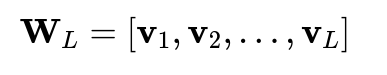
When we project these centroids using the LDA transformation matrix

, we get projected centroids

. In standard LDA, W has

columns, giving us projected centroids in

The Core Challenge: Projecting to L < K-1 Dimensions

When we need to project to

dimensions where

, we're essentially asking: "How can we preserve as much discriminative information as possible while reducing dimensionality below the theoretical maximum?"

This isn't just a mathematical curiosity—it has practical implications. Lower-dimensional representations are computationally efficient, less prone to overfitting, and often better for visualization. The challenge lies in selecting which dimensions to keep.

Eigendecomposition Approach with Practical Insights

The eigendecomposition of

gives us eigenvectors that define the discriminant directions in our feature space. These eigenvectors, ordered by their corresponding eigenvalues, represent directions of decreasing discriminative power.

To project to

dimensions, we select the

eigenvectors with the largest eigenvalues:

The projected centroids are then:

This approach is analogous to principal component analysis (PCA), but with a crucial difference: while PCA maximizes variance, LDA maximizes class separability. The eigenvalues in LDA directly quantify how much discriminative information each direction captures.

In practice, the first few eigenvectors often capture most of the discriminative information. This is why dimensionality reduction to

can be effective—we're keeping the most informative directions while discarding those that contribute little to class separation.

Optimization Perspective and Geometric Interpretation

From an optimization standpoint, we're solving:

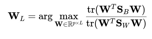
subject to

Geometrically, this means we're finding a subspace where the projected centroids are as far apart as possible (maximizing between-class scatter) while keeping the projected data points within each class as close together as possible (minimizing within-class scatter).

The trace ratio formulation provides an intuitive understanding: we're maximizing the ratio of between-class variance to within-class variance in the projected space. This directly aligns with Fisher's original criterion for discriminant analysis.

Implementation Considerations and Challenges

Handling Singular Within-Class Scatter Matrices

In high-dimensional spaces with limited samples,

often becomes singular, making its inverse undefined. This is a common challenge in LDA implementation. Several approaches address this:

Regularization adds a small constant to the diagonal:

This stabilizes the matrix inversion but introduces a hyperparameter

that needs tuning.

Alternatively, we can reformulate the problem as a generalized eigenvalue problem:

This avoids explicit matrix inversion and is numerically more stable.

Computational Efficiency for Large Datasets

For large datasets with high dimensionality, computing and storing the scatter matrices becomes expensive. A practical approach is to use a two-stage dimensionality reduction:

# Example: Two-stage dimensionality reduction for LDA
import numpy as np
from sklearn.decomposition import PCA
from sklearn.discriminant_analysis import LinearDiscriminantAnalysis

# First stage: PCA to reduce to a manageable dimension
pca = PCA(n_components=min(n_samples-1, n_features))
X_pca = pca.fit_transform(X)

# Second stage: LDA to project to L dimensions
lda = LinearDiscriminantAnalysis(n_components=L)
X_lda = lda.fit_transform(X_pca, y)

# To project centroids, first compute them in the original space
centroids = np.array([X[y == i].mean(axis=0) for i in np.unique(y)])

# Project centroids through PCA
centroids_pca = pca.transform(centroids)

# Project centroids through LDA
centroids_lda = lda.transform(centroids_pca)

This approach first reduces dimensionality using PCA (which preserves variance) and then applies LDA on the reduced space (which maximizes class separation).

Addressing Potential Follow-up Questions

How do you determine the optimal value of L?

The optimal value of L depends on your specific goals and dataset characteristics. Several approaches can guide this decision:

Cross-validation can empirically determine which L yields the best classification performance on held-out data.

Examining the eigenvalue spectrum helps identify where the "elbow" occurs—the point where additional dimensions contribute minimally to class separation.

Information-theoretic criteria like AIC or BIC can balance model complexity against goodness of fit.

In practice, I often plot classification performance against increasing values of L to find the point of diminishing returns.

How does this approach compare to other dimensionality reduction techniques?

Unlike unsupervised methods like PCA, t-SNE, or UMAP, LDA is supervised and specifically optimizes for class separability. This makes it particularly effective when the classification task is the primary goal.

However, LDA makes stronger assumptions than some methods—it assumes classes have equal covariance matrices and are approximately Gaussian distributed. When these assumptions are violated, kernel LDA or more flexible discriminant analysis variants might be preferable.

For visualization purposes (L=2 or L=3), t-SNE often produces more visually appealing clusters, but LDA projections typically preserve more of the original discriminative structure.

What if the classes are imbalanced?

Class imbalance affects LDA in two ways: it biases the global mean toward the majority class, and it gives more weight to the scatter of larger classes.

To address this, we can use weighted LDA, where each class contribution to the scatter matrices is normalized by its size:

# Example: Implementing weighted LDA for imbalanced classes
def weighted_scatter_matrices(X, y):
    classes = np.unique(y)
    n_classes = len(classes)
    n_features = X.shape[1]

    # Global mean
    global_mean = np.mean(X, axis=0)

    # Initialize scatter matrices
    S_W = np.zeros((n_features, n_features))
    S_B = np.zeros((n_features, n_features))

    for i, cls in enumerate(classes):
        X_cls = X[y == cls]
        n_samples = X_cls.shape[0]

        # Class mean
        mean_cls = np.mean(X_cls, axis=0)

        # Within-class scatter (normalized by class size)
        S_W_cls = np.cov(X_cls, rowvar=False) * (n_samples - 1) / n_samples
        S_W += S_W_cls

        # Between-class scatter (all classes contribute equally)
        mean_diff = mean_cls - global_mean
        S_B += np.outer(mean_diff, mean_diff)

    # Normalize between-class scatter by number of classes
    S_B /= n_classes

    return S_W, S_B

This approach ensures that all classes contribute equally to the discriminant directions, regardless of their size.

How does this extend to non-linear problems?

For non-linear class boundaries, kernel LDA extends our approach by implicitly mapping data to a higher-dimensional space where classes become linearly separable.

The kernel trick allows us to compute the scatter matrices in this implicit feature space without explicitly performing the mapping:

# Example: Kernel LDA implementation
def kernel_lda(X_train, y_train, X_test, L, kernel='rbf', gamma=1.0):
    from sklearn.metrics.pairwise import pairwise_kernels

    # Compute kernel matrix
    K = pairwise_kernels(X_train, metric=kernel, gamma=gamma)

    # Compute class-specific kernel matrices
    classes = np.unique(y_train)
    n_classes = len(classes)
    n_samples = X_train.shape[0]

    # One-hot encoding of labels
    Y = np.zeros((n_samples, n_classes))
    for i, cls in enumerate(classes):
        Y[y_train == cls, i] = 1

    # Class means in kernel space
    N = np.diag(1.0 / np.sum(Y, axis=0))
    M = Y @ N @ Y.T @ K

    # Center kernel matrix
    one_n = np.ones((n_samples, n_samples)) / n_samples
    K_centered = K - one_n @ K - K @ one_n + one_n @ K @ one_n

    # Between-class scatter
    S_B = M @ K_centered @ M.T

    # Within-class scatter (regularized)
    S_W = K_centered @ (np.eye(n_samples) - M) @ K_centered + 1e-10 * np.eye(n_samples)

    # Solve eigenvalue problem
    eigvals, eigvecs = np.linalg.eigh(np.linalg.inv(S_W) @ S_B)

    # Sort eigenvectors by eigenvalue in descending order
    idx = np.argsort(eigvals)[::-1]
    eigvals = eigvals[idx]
    eigvecs = eigvecs[:, idx]

    # Select top L eigenvectors
    W = eigvecs[:, :L]

    # Project test data
    K_test = pairwise_kernels(X_test, X_train, metric=kernel, gamma=gamma)
    K_test_centered = K_test - np.ones((X_test.shape[0], 1)) @ np.mean(K, axis=0).reshape(1, -1)

    return K_centered @ W, K_test_centered @ W

The centroids in kernel space are implicitly defined and projected through the same transformation as the data points.

Practical Applications and Insights

Beyond classification, this centroid projection approach has valuable applications in:

Transfer learning: Projecting centroids from a source domain to a target domain can help align feature spaces across domains.

Anomaly detection: The distance of a point to its projected class centroid in the L-dimensional space provides a measure of outlierness.

Interpretability: The reduced dimensions often have meaningful interpretations in terms of the original features, especially when L is small.

In my experience, the most powerful aspect of this approach is its ability to distill the essential discriminative information into a minimal representation. This not only improves computational efficiency but often enhances model generalization by focusing on the most robust discriminative patterns in the data.

Theoretical Guarantees and Limitations

It's worth noting that while projecting to L < K-1 dimensions necessarily loses some discriminative information, the eigendecomposition approach guarantees that we retain the maximum possible discriminative power for the given dimensionality L.

However, this optimality is with respect to the specific criterion (the Fisher criterion) and assumes that the class distributions are Gaussian with equal covariance matrices. When these assumptions are violated, the projections may be suboptimal.

In practice, I've found that even when assumptions aren't perfectly met, LDA projections still provide valuable dimensionality reduction, especially as a preprocessing step for other algorithms or for visualization purposes.

Connecting to Deep Learning Perspectives

Modern deep learning approaches to dimensionality reduction, like deep metric learning, can be viewed as non-linear extensions of the principles behind LDA. They learn embeddings that maximize between-class distances while minimizing within-class distances, but do so through neural networks rather than explicit matrix operations.

The centroid projection concepts we've discussed remain relevant even in these advanced contexts—many deep metric learning methods explicitly use class centroids in their loss functions or evaluation metrics.

# Example: Deep metric learning with centroid-based loss
import torch
import torch.nn as nn
import torch.nn.functional as F

class CentroidLoss(nn.Module):
    def __init__(self, num_classes, embedding_size):
        super(CentroidLoss, self).__init__()
        self.centroids = nn.Parameter(torch.randn(num_classes, embedding_size))

    def forward(self, embeddings, labels):
        # Calculate distance to centroids
        centroids = F.normalize(self.centroids, p=2, dim=1)
        embeddings = F.normalize(embeddings, p=2, dim=1)

        # Cosine similarity between embeddings and centroids
        cosine_sim = embeddings @ centroids.t()

        # Cross-entropy loss
        return F.cross_entropy(cosine_sim, labels)

This deep learning perspective brings us full circle—the fundamental principles of separating class centroids in a discriminative space remain central across classical and modern approaches.