ML Interview Q Series: Provide an analogy for a Cost Function in real life

📚 Browse the full ML Interview series here.

Comprehensive Explanation

A cost function in Machine Learning is a measure of how far off your model’s predictions are from the actual values in the training dataset. It quantifies the “error” of your model. In simpler terms, it is the number that you want to minimize when training your model, because reducing the cost function typically improves the model’s predictive accuracy.

A good real-life analogy is thinking of a cost function as the “penalty meter” or “dissatisfaction score” that accumulates every time you deviate from your goal. The aim is to reduce that dissatisfaction score to be as small as possible.

Imagine you are delivering packages to different locations in a city, and your objective is to do it in the shortest total distance traveled. Every extra mile you drive beyond some optimal route is like adding to the dissatisfaction score. You want to find the route that minimizes the total distance you drive (i.e., the total penalty). In a Machine Learning setting, each mile beyond the “ideal” route corresponds to an error between the model’s prediction and the actual label. By summing (or averaging) this error across all packages (training examples), you get a numerical value that indicates how well you are delivering packages overall. Minimizing it means you’re consistently delivering packages in the most efficient way possible, just like a machine learning model tries to minimize errors across the entire training dataset.

Mathematical Representation of a Cost Function

Below is one commonly used cost function (mean of the loss over all training samples). It is typically called the Mean Squared Error (MSE) in regression problems, or a generalized form of average loss in classification and other tasks:

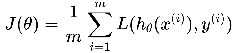
Here, m is the total number of training examples in your dataset. x^(i) represents the i-th input data point, y^(i) is the true label for that i-th data point, h_{theta}(x^(i)) is the model’s prediction for the i-th data point given parameters theta, and L(...) is the loss function that measures the discrepancy between the prediction and the actual label. The cost function J(theta) is simply the average of those losses across all training examples.

Code Example in Python

Below is a brief snippet of Python code (using standard numerical libraries) that demonstrates how you might compute an MSE-style cost function. This snippet assumes you have lists or arrays for predicted values (y_pred) and actual values (y_true):

import numpy as np

def mean_squared_error_cost(y_true, y_pred):
    # Ensure inputs are NumPy arrays
    y_true = np.array(y_true)
    y_pred = np.array(y_pred)

    # Calculate MSE
    mse = np.mean((y_true - y_pred) ** 2)
    return mse

# Example usage
y_true = [3.2, 5.1, 7.7, 9.0]
y_pred = [3.0, 4.8, 8.2, 9.3]

cost_value = mean_squared_error_cost(y_true, y_pred)
print("The cost (MSE) is:", cost_value)

How the Real-Life Analogy Relates to Minimizing the Cost

In the “delivery route” analogy, every extra unit of distance traveled contributes to the overall travel distance. If you measure your total distance after each delivery, that total distance is analogous to the cost function. By improving your path (choosing better model parameters in Machine Learning), you reduce your total distance (overall error). Over time, you’ll keep refining your route (train your model) to minimize the distance traveled (cost function).

Potential Follow-up Questions

Can you explain the difference between a Cost Function and a Loss Function?

A loss function measures the discrepancy between your model’s prediction and the true label for a single data point. A cost function, on the other hand, is typically the average of those loss values across the entire training set. In other words, the cost function aggregates (or averages) individual loss measurements to give an overall sense of the model’s performance on all training examples. Sometimes the terms cost function and loss function are used interchangeably, but the general convention is that the loss function applies at a single sample, and the cost function is the overall (or average) loss across all samples.

What are some different cost functions, and when would you use them?

There are many types of cost functions, each suited for specific tasks. For regression, Mean Squared Error (MSE) is common. For classification, Cross-Entropy is popular. Huber Loss can be used in regression tasks that need to be more robust against outliers. The choice depends on the nature of your problem—if you are dealing with continuous values, MSE or Mean Absolute Error can be a good start. For classification, you often use log loss or cross-entropy. Each type of cost function encodes different assumptions and priorities about errors. For instance, MSE penalizes large errors more severely because squaring the difference emphasizes outliers, whereas Mean Absolute Error penalizes all deviations linearly.

How do you handle imbalanced classes in your cost function?

In the case of severe class imbalance, a standard cost function like plain cross-entropy might not be sufficient. You would need to adjust the loss function to pay more attention to the minority class. Techniques like Weighted Cross-Entropy or Focal Loss can be used, where you modify or add factors to the loss function to counteract the imbalance. Class-weighting, sampling methods, or using specialized loss functions can help the model focus on the underrepresented classes.

How do you ensure your cost function is differentiable for gradient-based methods?

Most gradient-based optimizers assume differentiability of the cost function. Commonly used cost functions like MSE and cross-entropy are differentiable in terms of the model parameters. If you use a custom cost function that is not differentiable everywhere (for instance, an absolute value term introduces a point of non-differentiability at 0), many optimizers can handle it with subgradient techniques. However, it can sometimes complicate training or result in slower convergence, so most practical ML implementations rely on smooth cost functions.

Does minimizing a particular cost function always guarantee the best real-world performance?

Minimizing the cost function leads to an optimal solution with respect to that particular metric. However, the chosen cost function might not fully capture your real-world objectives. For example, if your actual goal is to maximize user satisfaction, or to optimize for recall at the expense of precision, a standard cost function like MSE might not reflect that real-world trade-off. You might need to select or design a cost function more aligned with your practical goals, or use additional metrics like F1 score, precision-recall, or domain-specific evaluation measures to ensure you are indeed optimizing for the right objectives.

Below are additional follow-up questions

How can we distinguish between the training cost and the test cost, and why is this distinction important?

In Machine Learning, the training cost refers to the performance of your model on the training data. The test cost is the error measure on previously unseen data, generally referred to as the test or validation set. When you train a model, you typically optimize for the training cost by adjusting parameters until the training loss is minimized. However, if the model becomes too attuned to the training examples (i.e., it memorizes the data rather than generalizing), you risk overfitting. Overfitting can be detected when the training cost is very low but the test cost remains high or starts increasing as training continues.

A potential pitfall is ignoring signs of overfitting, such as a large disparity between training cost and test cost. This can happen if the model has too many parameters compared to the amount and complexity of data. A common real-world issue is that project timelines may focus solely on training metrics without giving enough attention to test metrics, leading to a model that fails to perform well on unseen data.

What happens if the cost function you’re using has multiple local minima, and how could you address such an issue?

Some cost functions, especially those encountered in Deep Learning, are non-convex and can contain multiple local minima or saddle points. This occurs because neural networks with multiple layers have highly complex error surfaces. Getting stuck in a local minimum means the optimization algorithm might converge to a suboptimal point instead of the global minimum.

One way to address this is by using algorithms or techniques that help escape local minima or saddle points, such as stochastic gradient descent with momentum or Adam. The randomness introduced by mini-batch updates, as well as the momentum that can push the parameters out of shallow local minima, can help the model find better regions of the parameter space. Another approach is to perform multiple random restarts or incorporate learning rate schedules.

A subtle real-world concern is that, in very high-dimensional parameter spaces, local minima are actually less problematic than saddle points, where gradients are small in some directions and large in others. Ensuring that the optimization algorithm can progress even when gradients are tiny is a key design consideration.

How do we handle scenarios where the cost function is non-convex?

Many real-world cost functions—especially in Deep Learning—are inherently non-convex. This means that there is no guarantee that gradient descent or similar methods will find a unique global minimum. Nonetheless, practical experience has shown that neural networks often yield good performance despite non-convexity. Modern optimizers like Adam, RMSProp, and even simple stochastic gradient descent tend to find solutions that generalize well if hyperparameters (like learning rate and batch size) are tuned effectively.

An important edge case is when hyperparameters are not well chosen. For example, a learning rate that is too large may cause the model to diverge or bounce chaotically around the parameter space, while a learning rate that is too small can lead to very slow convergence or entrapment in suboptimal regions. Another subtlety arises when the dataset distribution is constantly changing (e.g., streaming data or non-stationary contexts), which can make non-convex optimization even more challenging because the cost function is effectively shifting over time.

Can a cost function have multiple objectives, and how do we balance them?

It is entirely possible to have multiple objectives in a single cost function. This scenario is often referred to as multi-objective optimization. A common example in supervised learning is combining a primary objective (like minimizing MSE) with a regularization term (like L2 regularization) to prevent overfitting. Instead of optimizing a single measure of accuracy, you optimize a weighted sum of accuracy and a complexity penalty.

Balancing these objectives involves selecting appropriate weighting factors. If the regularization coefficient is too high, you might underfit because you heavily penalize large parameter values. If it’s too low, you risk overfitting by not penalizing complexity enough. This trade-off can be tricky to fine-tune in real-world settings, particularly when the data is noisy or the resource constraints (like memory and compute) are stringent. In advanced scenarios, you might have more than two objectives (for instance, cost, latency, and fairness). One pitfall in these cases is ignoring the potential interactions between the different objectives, such as improving speed at the expense of significantly harming accuracy.

What if the cost function is not well-defined or becomes undefined for certain data points?

In some cases, the cost function might involve terms that become undefined for certain inputs. For example, a log loss (as used in cross-entropy) becomes undefined if a model predicts a probability of zero for a class that actually occurs. This can create numerical stability issues, such as NaN (Not a Number) values in your training process.

A practical solution is to add small numeric values (like epsilon) to prevent taking the log of zero. For example, you might replace log(p) with log(p + epsilon). A subtle real-world pitfall is failing to realize that some transformation in your input pipeline might generate out-of-bound predictions. If you are using normalization layers or have unbounded parameter updates, the model might produce numeric overflow or underflow. Proper data preprocessing and parameter initialization are essential to avoid these problematic edge cases.

How does the gradient of the cost function guide the optimization, and what if the gradient is very large or very small?

In gradient-based methods, the gradient of the cost function with respect to model parameters indicates the direction of steepest ascent in cost space. In practice, we move in the opposite direction (steepest descent) to reduce the cost. The magnitude of the gradient can also signal how big a step you should take in updating parameters. If the gradient is too large, you risk unstable updates (sometimes called “exploding gradients”), causing erratic parameter jumps. If the gradient is too small (“vanishing gradients”), learning stalls and parameters barely change.

Many real-world issues arise from exploding or vanishing gradients, particularly in deep neural networks. Techniques such as gradient clipping can tame exploding gradients. Architectural changes like LSTM or GRU units can mitigate vanishing gradients in recurrent networks. Careful initialization and normalization (e.g., batch normalization) can also help keep gradients within a manageable range.

In practice, how can a custom cost function be implemented in frameworks like PyTorch or TensorFlow, and what are common pitfalls?

When implementing a custom cost function in PyTorch or TensorFlow, you usually define a function that computes the error term based on your model’s predictions and labels. Then, the framework’s automatic differentiation engine calculates gradients for you. A typical code snippet in PyTorch might look like this:

import torch

def custom_loss(predictions, targets):
    # predictions and targets are torch tensors
    # shape: (batch_size, num_classes) or similar
    # Implement your custom logic here
    error = (predictions - targets) ** 2
    return torch.mean(error)

# Example usage in a training loop
optimizer = torch.optim.SGD(model.parameters(), lr=0.01)

for data, labels in dataloader:
    optimizer.zero_grad()
    outputs = model(data)
    loss = custom_loss(outputs, labels)
    loss.backward()
    optimizer.step()

One subtle edge case is ensuring that the tensor operations you perform are differentiable. If you introduce non-differentiable operations or pythonic control flow that breaks the gradient path, you may find that no gradients are calculated for certain parameters. Another common pitfall is mismatching tensor shapes or forgetting to move tensors to the correct device (CPU vs. GPU). These framework-specific nuances can lead to silent errors or unexpected results if not handled carefully.