
ML Interview Q Series: Random Permutation Switches: Constant Expected Value (1/2) via Indicator Variables.
Browse all the Probability Interview Questions here.
Question: Take a random permutation of the integers 1, 2, ..., n. Let us say that the integers i and j with i ≠ j are switched if the integer i occupies the jth position in the random permutation and j occupies the ith position. What is the expected value of the total number of switches?
Short Compact solution
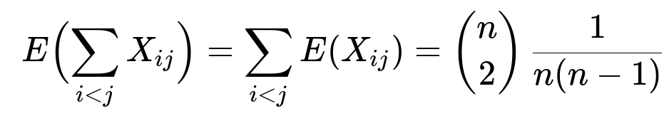
Define an indicator variable X_ij = 1 if i and j (with i < j) are switched and 0 otherwise. Note that the probability that i and j are switched is 1/[n(n-1)] because out of n! total permutations, exactly (n-2)! permutations place i in position j and j in position i. Therefore, E(X_ij) = 1/[n(n-1)]. Summing this expectation over all distinct unordered pairs (i, j) (of which there are n choose 2) yields:
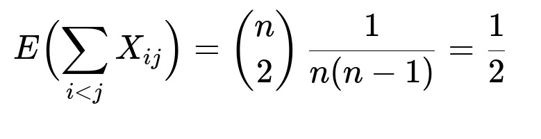
Hence, the expected number of switches is always 1/2, regardless of n.
Comprehensive Explanation
Indicator Variable Setup
We have a random permutation of {1, 2, ..., n}. A switch occurs if two distinct elements i and j occupy each other’s positions in the permutation. In other words:
i goes to position j,
j goes to position i.
To handle these events mathematically, we introduce X_ij, an indicator random variable defined for each pair i < j:
X_ij = 1 if i and j are switched,
X_ij = 0 otherwise.
The total number of switches in the permutation is then the sum of these indicators over all distinct pairs i < j: total number of switches = sum_{i<j} X_ij.
Probability That X_ij = 1
We want to find P(X_ij = 1). For i and j to be switched, i must occupy position j and j must occupy position i. In a random permutation of n distinct elements:
There are n! total permutations.
Fixing i → j and j → i is equivalent to reducing the permutation problem to permuting the remaining n - 2 elements arbitrarily in the remaining n - 2 positions.
The number of ways to permute the remaining n - 2 elements is (n - 2)!.
Thus P(X_ij = 1) = (n - 2)! / n! = 1/[n(n-1)].
Expected Value of X_ij
Since X_ij is an indicator random variable, E(X_ij) = P(X_ij = 1). Hence:
E(X_ij) = 1/[n(n-1)].
Summing Over All Pairs
There are n choose 2 distinct pairs (i, j) with i < j. By linearity of expectation, the expected number of switches is:
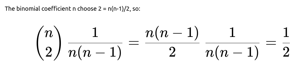
Thus, the expected total number of switches in a random permutation of n elements is always 1/2.
Potential Follow-Up Questions
Why does this expected value not depend on n?
Even though there are more possible pairs as n grows larger, the probability that any specific pair (i, j) is switched shrinks at exactly the same rate (1/[n(n-1)]). The two factors (increasing number of pairs vs. decreasing probability) cancel each other out. Hence, the product remains 1/2 regardless of n.
Can we confirm this result through a quick simulation in Python?
Absolutely. Here is a simple Python snippet that approximates the expected number of switches for different values of n:
import random
import statistics

def count_switches(perm):
    switches = 0
    for i in range(len(perm)):
        # The elements are 1-indexed conceptually, but Python lists are 0-indexed
        # We'll adjust carefully:
        elem_i = perm[i]   # the integer in position i (0-indexed)
        # position i in 1-indexed sense is i+1
        # so we check if perm[i] == j and perm[j-1] == i+1 in 1-based
        # but to keep it simpler, we do direct condition below:
        for j in range(i+1, len(perm)):
            elem_j = perm[j]
            # i, j are positions in 0-based. The integers are 1-based stored in perm.
            # we say i and j are switched if integer i+1 occupies j+1 position
            # AND integer j+1 occupies i+1 position
            if elem_i == (j+1) and elem_j == (i+1):
                switches += 1
    return switches

def simulate_switches(n, trials=10_000):
    results = []
    for _ in range(trials):
        perm = list(range(1, n+1))
        random.shuffle(perm)
        results.append(count_switches(perm))
    return statistics.mean(results)

for n in [2, 3, 5, 10, 50, 100]:
    print(f"n={n}, Estimated E[# of switches] = {simulate_switches(n):.4f}")
When you run this, you would see that the average number of switches rapidly converges to ~0.5 as the number of trials grows.
What if we were asked for the variance of the total number of switches?
We would need to compute Var(sum_{i<j} X_ij). Because indicator variables can be correlated (switching a pair (i, j) might subtly influence the probability that another pair (k, l) is also switched), one must consider both E(X_ij) and E(X_ij X_kl) for i < j, k < l. This is a more involved calculation requiring careful combinatorial arguments. However, the key takeaway is that while the expected value is surprisingly simple, the variance computation requires accounting for intersections among events of different pairs.
How do we interpret “switches” in the language of cycle decomposition?
In cycle notation for permutations, a switch of i and j alone corresponds to a 2-cycle (also called a transposition if we treat it independently, but specifically here it’s a 2-cycle embedded in the entire permutation). The question effectively asks: “What is the expected number of disjoint 2-cycles in a random permutation?” The result that the expected number of 2-cycles is 1/2 aligns with known results in the theory of random permutations, where the expected number of r-cycles is 1/r.
Does this concept generalize to detecting “r-cycles” in random permutations?
Yes. In general, the expected number of r-cycles in a random permutation of n elements is 1/r. Here, the r=2 case (2-cycles) happens to correspond exactly to these “switch” events. For r=3, the expected number of 3-cycles would be 1/3, and so on, provided n is large enough to accommodate cycles of length r.
What if i = j were allowed?
In the question, i ≠ j is explicit, so we never consider i = j. If i = j, that would not make sense as a “switch” because it would require the same element to go to a different position and simultaneously remain in its own position. Hence i = j is excluded.
How is this relevant to real-world data engineering or ML system design?
When data transformations are applied randomly, it’s sometimes crucial to estimate how many elements return to specific positions or exchange positions. A confusion between labeling and indexing can be spotted or estimated using approaches like these.
The concept of indicator variables and linearity of expectation is pervasive in analyzing randomized algorithms, hashing, or random indexing.
Knowing that the expected value is 1/2 no matter how large n gets can inform us that certain pairwise “swap events” remain vanishingly likely for each pair as n increases, but the sheer number of pairs compensates exactly to keep a constant expected total.
These follow-up discussions confirm mastery of the underlying probability principles and the broader connections to random permutations in mathematics.
Below are additional follow-up questions
What if we define a “switch” only as one-directional? For instance, i lands in position j, but j is not necessarily in position i.
A one-directional scenario changes the definition of the event significantly. If “switch” is no longer strictly mutual and we only require i to be in position j (without j being in i’s position), then each pair i, j can have multiple ways to occur. Specifically:
For i to land in position j, we only constrain that one of the permutation’s slots is fixed, leaving the remaining n-1 positions for the other elements.
The condition does not require j → i, so j can appear in any other position.
Consequently, the probability that i is in position j alone is 1/n for a uniform random permutation. Summing over all pairs (i, j) with i ≠ j would be n(n - 1) * (1/n) = n - 1, so the expected count of one-directional placements i → position j is n - 1. This result is substantially different from 1/2. A key pitfall is conflating the original two-way definition with a single-direction event, which can lead to an incorrect application of the 1/[n(n-1)] probability logic.
What if the permutation is drawn from a non-uniform distribution?
When permutations are not chosen uniformly at random, the probability P(X_ij = 1) can deviate from 1/[n(n-1)]. For example, if the distribution favors permutations where indices and elements are “close” to each other (or, conversely, permutations that maximize dislocation), then pairs (i, j) might have a different probability of being switched. A typical pitfall is to assume uniformity when, in real data or certain sampling methodologies, permutations might be biased (e.g., “nearly sorted” permutations are more common). In such cases, one must explicitly compute or estimate P(X_ij = 1) under the new distribution. The linearity of expectation still holds, but the probability must be derived carefully for the given bias.
How does the concept of “switches” compare to the concept of “inversions” in permutations?
An inversion is typically defined as a pair (i, j) such that i < j but the position of i is to the right of the position of j in the permutation. A “switch,” as defined here, specifically requires i and j to occupy each other’s positions. While both concepts involve pairs and positions, a switch is a much stricter condition (i → j and j → i). A potential pitfall is confusing these two definitions. The expected number of inversions in a random permutation of n elements is n(n-1)/4, which is substantially larger than 1/2 for the expected number of two-way switches. Hence, using the inversion formula or logic in place of switch-based reasoning would be incorrect.
What if elements are not all distinct? For instance, if some values are repeated?
The concept of “switching” i and j fundamentally relies on distinct labels i and j to track positions. If there are repeated elements, then labeling becomes ambiguous: two identical elements cannot be distinguished by their numeric label i or j. This ambiguity means that “i occupies j’s position” and “j occupies i’s position” might no longer be well-defined. In practice, one might have to tag identical elements with auxiliary labels (like ID numbers) to define what “switched” means. A subtle pitfall is failing to assign unique labels to repeated elements, which makes the probability calculation for X_ij ill-defined.
What if we only consider a partial permutation of k out of n elements?
A partial permutation (also known as a k-permutation of n) is a selection of k distinct elements arranged in k of the n positions, leaving the remaining n - k positions unoccupied or irrelevant. In such cases, the definition of “switch” would only apply to those chosen k elements. The probability that two of the chosen elements end up mutually swapped depends on how the partial permutation is sampled:
If we first choose which k elements will be in use and then permute them uniformly among the k chosen positions, the probability that a particular pair is swapped changes relative to the full n-element scenario because the sample space is smaller.
The expected number of switches among those k chosen elements would still involve an indicator approach but would now sum over the pairs among the k selected elements. The exact probability P(X_ij = 1) = 1/[k(k-1)] if i and j are among the chosen set and placed in k distinct positions.
A pitfall arises if one attempts to reuse the 1/[n(n-1)] logic directly without adjusting for the reduced sample space of partial permutations.
Can two different pairs of elements overlap in their switching? For example, can (i, j) and (j, k) both be switches simultaneously?
In theory, for i, j, k distinct from each other, the event “i and j are switched” means i → j and j → i, while the event “j and k are switched” means j → k and k → j. Both cannot be satisfied simultaneously if i, j, k are distinct, because j cannot occupy two different positions. Hence, some overlap events in the sum of indicators are impossible. This highlights that certain pairs of events are mutually exclusive, while others might have more subtle correlations. A common pitfall is forgetting that X_ij and X_jk might have zero or nonzero correlation depending on whether the sets {i, j} and {j, k} can simultaneously be involved in distinct switches. This overlap is an important detail if one wants higher moments (like variance or covariance) but does not affect the linearity-of-expectation argument for the mean.
What does the distribution of the total number of switches look like, beyond just its expectation?
While the expected number of switches is 1/2, the full distribution of the random variable sum_{i<j} X_ij is skewed heavily toward values 0 or 1. In fact, having even two distinct pairs simultaneously switched would require at least four distinct elements occupying each other’s positions two by two, which is a rarer event. The pitfall here is to assume that the value must center heavily around 1/2 or that the variance is small; actually, the distribution is quite sparse (it is quite likely to be 0 or 1, with lower probabilities assigned to higher counts). A more detailed combinatorial analysis is required to see exactly how the mass spreads out.
How might “switches” manifest in a real-world data pipeline, for instance, in data shuffling for training?
If we consider a data pipeline that shuffles indices of a dataset, a “switch” between indices i and j means that the sample originally intended for position i ends up at position j, and vice versa. In real-world systems, we typically want robust shuffles that do not systematically bias the model toward certain data orders. The negligible expected number of mutual swaps (1/2) might sound inconsequential; however, even one such swap might cause confusion if the pipeline relies on strict indexing for labels or for specific transformations. A subtle pitfall is assuming “small expected number” implies “no big deal,” without considering that even one or two such swapped pairs could cause indexing logic errors or mislabeled data if the rest of the pipeline is not designed to handle them.
Could there be a combinatorial identity hidden behind the result E[# of switches] = 1/2?
Indeed, the identity arises from summing 1/[n(n-1)] over all n(n-1)/2 pairs. This can be recognized as a particular instance of a more general identity involving cycle counts in permutations, or as a direct combinatorial argument about how each pair i, j can be arranged. The deeper combinatorial perspective sees each pair of positions as having a 1/n(n-1) chance to be a 2-cycle in the permutation. A pitfall might be to treat the result as purely coincidental without realizing it reflects a broad principle: the expected count of r-cycles in a random permutation of n distinct elements is 1/r. That “1/2” for 2-cycles is just a specific instance of that principle.
How does the result change if we allow permutations to be constructed incrementally, placing one element at a time?
When constructing a permutation incrementally, we might place each element i in a randomly chosen unoccupied position among the available slots. The probability analysis for a final arrangement remains the same once all elements are placed, because this incremental process is just another way to sample a uniform permutation (if every partial selection is equally likely). Hence the final distribution of permutations does not change. A pitfall could be to think the step-by-step approach modifies the chance that i → j and j → i occur, but as long as each final permutation remains equally likely, the expectation E[# of switches] still equals 1/2. However, if the incremental placement is biased (e.g., we choose positions with varying probabilities at each step), then uniformity fails and the previously derived 1/2 result no longer holds.