
ML Interview Q Series: Random String Tying: Expected Loops Through Recurrence and Harmonic Series.
Browse all the Probability Interview Questions here.
A bin contains N strings. You randomly choose two loose ends and tie them up. You continue until there are no more free ends. What is the expected number of loops you get?
Short Compact solution
We let Xn be the random variable denoting the number of loops produced by n strings. We also define an indicator Yn = 1 if the first pair of ends we tie belong to the same string, and 0 otherwise. By the law of total expectation:
$$ E(X_n) = E(X_n \mid Y_n = 1),P(Y_n = 1) ;+; E(X_n \mid Y_n = 0),P(Y_n = 0)
= \bigl[1 + E(X_{n-1})\bigr]\frac{1}{2n-1} ;+; E(X_{n-1})\Bigl(1 - \frac{1}{2n-1}\Bigr) = \frac{1}{2n-1} + E(X_{n-1}). $$
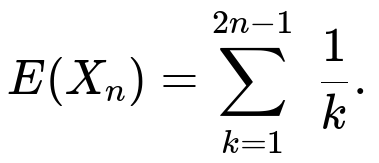
Solving this recurrence with the base case E(X0) = 0 yields:
Comprehensive Explanation
Setup and Reasoning
When we have n strings, there are in total 2n loose ends. If we randomly select two ends to tie together, there is a 1/(2n - 1) chance that these two ends belong to the same string. Tying two ends of the same string forms a loop immediately, and it also effectively reduces the problem from n strings to n - 1 strings (because we have created one closed loop and are left with one fewer “active” string).
If, on the other hand, the chosen ends belong to different strings (which happens with probability (2n - 2)/(2n - 1)), those two strings become joined into one longer string. We still proceed with the same overall problem, but we do not gain an immediate additional loop from that particular tie.
Hence, denoting Xn as the expected number of loops with n strings:
With probability 1/(2n - 1), we tie ends of the same string, creating a new loop plus the remainder’s expected loops is Xn-1.
With probability (2n - 2)/(2n - 1), we tie ends of different strings, and the expected loops remain Xn-1 without the extra loop.
So, E(Xn) = [1 + E(Xn-1)](1/(2n - 1)) + [0 + E(Xn-1)]((2n - 2)/(2n - 1)) = (1/(2n - 1)) + E(Xn-1).
This is a very simple recurrence:
E(Xn) - E(Xn-1) = 1/(2n - 1),
with E(X0) = 0. Summing these increments telescopes:
E(Xn) = 1/1 + 1/2 + 1/3 + … + 1/(2n - 1).
Thus, the expected number of loops is the (2n - 1)th harmonic number (minus any constant offsets, but here we start from 1/1 up to 1/(2n - 1) exactly).
Why the Probability of Tying Ends from the Same String is 1/(2n - 1)
Among 2n loose ends, choose one end arbitrarily (no restriction). There remain 2n - 1 ends that could be chosen as the second end.
Exactly 1 out of those (2n - 1) ends belongs to the same string (because each string has exactly 2 ends, so once you pick 1 end from a string, only 1 matching end from that same string is left).
Therefore, probability = 1/(2n - 1).
Intuitive Understanding
Each tie you make either closes a loop (if it happens to connect ends of the same string) or merges two strings. The chance of closing a loop each time shrinks in a particular harmonic-series pattern, resulting in the sum of reciprocal terms. Over the entire random tying process, it turns out you gain about log(2n) loops on average, since the harmonic series grows roughly like ln(2n).
Follow-Up Question 1: How does this expected number behave for large n?
For large n, the sum of 1/k from k=1 to k=2n-1 is approximately ln(2n-1) + γ, where γ is the Euler–Mascheroni constant (~0.5772...). Hence, for large n, E(Xn) grows on the order of ln(n). Concretely, we can say:
E(Xn) ~ ln(2n) + γ.
This indicates that even though you have n strings, on average you only end up with about ln(n) loops when you tie everything together randomly.
Follow-Up Question 2: How would you simulate this process in Python to empirically verify the result?
One straightforward approach is:
Represent each string by two free ends, labeled for convenience.
At each step, pick two free ends uniformly at random, tie them together, and check if they came from the same string or not.
Keep track of how many loops you form, then reduce or merge string identifiers accordingly.
Repeat until no free ends remain.
Average the result over many trials.
Below is a sketch:
import random
import statistics

def simulate_loops(n, trials=100000):
    results = []
    for _ in range(trials):
        # Represent each end as (string_id, end_id)
        # string_id in range(n), end_id in {0,1}
        ends = [(i, j) for i in range(n) for j in range(2)]
        # Keep track of which ends belong to which string
        # We can maintain a "parent" representative to merge strings
        parent = list(range(n))  # union-find or simple merges

        def find(x):
            # Path compression
            if parent[x] != x:
                parent[x] = find(parent[x])
            return parent[x]

        def union(a, b):
            pa, pb = find(a), find(b)
            if pa != pb:
                parent[pb] = pa

        loop_count = 0

        while len(ends) > 0:
            # Pick two ends
            e1 = ends.pop(random.randrange(len(ends)))
            e2 = ends.pop(random.randrange(len(ends)))
            s1, _ = e1
            s2, _ = e2
            root1, root2 = find(s1), find(s2)
            if root1 == root2:
                # same string -> forms a loop
                loop_count += 1
            else:
                # unify them into one string
                union(s1, s2)

        results.append(loop_count)
    return statistics.mean(results)

# Example usage:
for n in [1, 2, 5, 10, 50]:
    print(n, simulate_loops(n, trials=10000))
By comparing the output to the theoretical sum of 1/k for k=1..(2n - 1), you can see that the empirical averages align quite well with the theoretical expectation.
Follow-Up Question 3: Does the distribution of lengths of the strings matter for this expectation?
Interestingly, the initial lengths of the strings do not affect the expected number of loops, as long as there are n “active strings” each with 2 distinct ends. The process only cares that there are 2n total ends. The random tieing probabilities hinge on the total number of free ends and not on the internal structure/length of each string. Hence, the expected value result holds regardless of how the strings themselves are distributed in length.
Follow-Up Question 4: What is the variance of the number of loops?
While the expected value is relatively straightforward, the variance requires a bit more involved calculation. One standard way is to define Xn in terms of indicator random variables for whether each tie eventually closes a loop, then use E(Xn2) - [E(Xn)]2. The variance for this problem has been explored in various probability texts, but the final result involves harmonic number terms as well. The exact formula is more complicated, often including partial sums of reciprocals squared. You can derive it by carefully analyzing all pairwise covariances of indicators, or refer to known references on the “random pairing model” or “random matching problem.”
Follow-Up Question 5: Could we extend this idea if each string had more than two free ends initially?
Yes. If each “object” had m free ends and you randomly picked any two free ends to tie them together, the problem generalizes, but the probability that you form a “closed loop” in a single step changes. The recurrence relation would be different, because now each object has m free ends. Once you pick one end, there are (m n - 1) other free ends, of which (m - 1) belong to the same object. The same principle of total expectation can be applied, but you would carefully adjust the probabilities and the reduction from n to n-1 objects might not always be straightforward (particularly if objects can break into multiple loops). However, similar approaches—defining suitable indicator variables and applying the law of total expectation—often still apply.
Follow-Up Question 6: Are there real-world applications of this random tying problem?
Yes. This model has connections to:
Random matching or random pairing algorithms in combinatorics.
Problems in theoretical computer science involving random linkages or random permutations.
Certain interpretations of random chord models, like the “broken stick” problem in geometry or random chord problems in topology.
Simulation for “cords” in molecular or polymer-like structures.
While it might appear like a puzzle, understanding how randomness shapes “connectedness” or “closed loops” is fundamental in many statistical physics and combinatorial applications.
By mastering both the derivation of the expected number of loops and its real-world analogs, a candidate demonstrates thorough knowledge of applying probability theory, the law of total expectation, and combinatorial reasoning to solve non-trivial questions.
Below are additional follow-up questions
1) How does the order in which we tie ends affect the final count of loops, if at all?
One might wonder whether the specific sequence of random ties influences the expected number of loops. In other words, if we reorder the sequence of pairs we tie but still pick among all possible pairs uniformly, does it change the final expected loop count?
Detailed Explanation
Independence of Order Despite the fact that each tie reduces the number of free ends, the essence of the problem is that at each step you pick any two free ends uniformly at random. This uniformity means that no matter how you rearrange or label the sequence of steps, each pair selection is an equiprobable event among the remaining ends. Hence, from an expectation standpoint, the final count of loops does not depend on the temporal order of the ties as long as each step is random.
Formal Reasoning You can prove this by backward induction or by noting that we can treat the entire random process as a random matching on a set of 2n ends. Regardless of the order in which we “reveal” the edges of this matching, we are constructing the same random object. So, the expected value stays the same.
Potential Pitfall One subtlety is if your selection mechanism at each step is not truly uniform over all free ends (for example, if you skip certain pairs or prefer certain pairs). That non-uniform selection would change the probability structure and could thus change the expected number of loops. So, the “order doesn’t matter” statement only holds under fully uniform random selection at each step.
2) Is there a closed-form expression for the probability that exactly k loops are formed?
We know the expected number of loops, but the probability distribution over the number of loops is more complicated. One might ask for a closed-form or at least a known formula for P(Xn = k).
Detailed Explanation
Distribution Complexity The event of having exactly k loops is tied to how many times you select ends of the same string during the entire random matching process. A direct combinatorial argument might involve counting how many ways to partition 2n ends into matchings with a certain number of loops. This typically involves Stirling numbers or other advanced counting techniques.
Known Results The exact distribution can be expressed in terms of various combinatorial sums over matchings (sometimes called “one-factorizations” or “pairings”). There are known enumeration formulas for the number of ways to obtain exactly k cycles in a random permutation or pairing, but they are not usually as simple as a single closed-form expression for general n and k. The probability expression often requires summing complicated terms.
Potential Pitfall People sometimes assume that the distribution might be approximately normal for large n. While there might be a central limit theorem argument for the scaling of Xn, the leading behaviors can be somewhat subtle. Careful asymptotic analysis is required to confirm normal approximation or other limit theorems, and it is not as straightforward as the expectation alone.
Edge Cases
k=1: This is the probability that you end up with exactly one giant loop containing all 2n ends. This event is quite small for large n, but its exact probability can be computed from standard results on the number of ways to form a single cycle in a pairing.
k=n: This scenario implies that each tie connected the ends of the same string every single time, so you formed a loop at every step. This is extremely improbable but combinatorially possible if each random tie happens to select the matching end from the same string every time.
3) How do we interpret the process if we allow partial ties or re-tying (untying and re-tying ends)?
In some real-world scenarios, we might tie two ends and then later decide to untie or rearrange. One might ask whether this changes the expected number of loops formed by the end.
Detailed Explanation
Classical Simplification The standard version of the problem assumes that once two ends are tied, they remain tied. That means the total number of free ends continuously decreases by 2 until it reaches zero.
Impact of Untying If you allow untying, you effectively reintroduce free ends back into the system. This means the process is no longer a simple random matching among the original 2n ends. Instead, it becomes a more complicated stochastic process involving transitions from smaller to larger sets of free ends.
Expected Loop Count Changes Once untying is allowed, you lose the nice property that each step is a final, irreversible action. The expected number of loops by the end depends on the distribution of how many and which ties get undone. If untying is equally random or occurs with some probability, you might need to resort to Markov chain models that track the state (which ends are tied to which) over time. The end-of-process loop count can be significantly altered.
Potential Pitfall It is tempting to think you can just track net ties. However, the path by which ties are formed or undone influences the structure of the final arrangement. Merely counting net ties won’t suffice because re-tying can cause reconfiguration of loops in non-trivial ways. Thus, any form of partial tying or untying changes the underlying combinatorial framework drastically.
4) What if we tie more than two ends together at the same time (e.g., picking three or four ends and merging them into a node)?
In some generalizations, you might not just tie pairs but attempt to tie multiple ends together in a single step. For instance, you might pick four ends and tie them all at a single point.
Detailed Explanation
Traditional vs. Multi-Way Ties The classical problem is fundamentally about a perfect matching of 2n ends. But if you decide to pick four ends at a time and tie them all in one “knot,” you no longer have pairs forming edges in a graph. Instead, you create hyperedges or multi-way connections.
Graph/Hypergraph Interpretation
Pairwise ties naturally correspond to edges in a graph, leading to loops that correspond to cycles in that graph.
If you tie multiple ends together in one step, the structure is more akin to a hypergraph, and loops are not as straightforward to define. For example, tying four ends in one step might produce certain “closed components” that count as loops but can also yield substructures that are not loops in the standard sense.
Expected Number of Loops We must first define what constitutes a “loop” in this multi-way scenario. You could define a loop as any closed chain that you can form by traversing the multi-way nodes. However, the probability analysis changes substantially, and the direct 1/(2n-1) argument no longer holds. This would require a brand-new combinatorial approach or a Markov chain perspective with states describing how many multi-nodes currently exist.
Potential Pitfall If you conflate multi-end knots with pairwise ties, you might incorrectly apply the original formula. Each multi-end tie changes the number of remaining free ends differently and also can create multiple loops at once. So you must carefully re-derive or reconstruct the expected loop calculation from first principles.
5) How does this problem connect to random permutations or random matchings more formally?
In combinatorics, you can represent a random matching as a particular kind of permutation. One might wonder if there is a direct link between “tying ends” and “cycles in a random permutation.”
Detailed Explanation
Random Matchings vs. Random Permutations A permutation of 2n distinct elements can be decomposed into cycles. A perfect matching on 2n labeled points can also be viewed in relation to certain permutations—though typically, a matching is a fixed-point-free involution (i.e., a permutation that is its own inverse and has only cycles of length 2).
Relating Loops to Cycles In the classical problem, a “loop” corresponds to having a cycle in the underlying structure of how you match ends. However, each cycle in a random permutation is not always length 2, so you have to be precise: Tying ends in pairs is specifically a random involution, not a general permutation. The structure of cycles in that involution can be connected to the loop formation.
Known Theorems It is well-known that a random permutation of size n has an expected number of cycles that is Hn, the nth harmonic number. For a random involution on 2n elements, the expected number of cycles is also related to partial harmonic sums. This links directly to the sum from k=1 to 2n-1 of 1/k.
Potential Pitfall Confusion arises if you try to treat a random matching as an arbitrary random permutation with 2n elements. A random matching is only a subset of all permutations (specifically those that are perfect involutions). That is why we get a partial harmonic sum (up to 2n-1) instead of the full sum up to 2n. One must carefully distinguish a matching from a general permutation to avoid mixing up the respective cycle properties.
6) What is the time complexity or computational challenge in simulating this process for large n?
If you want to empirically validate the expected number of loops for very large n, or collect distribution data, you need an efficient algorithm.
Detailed Explanation
Naive Simulation A naive approach picks two ends at random among the free ends, merges them if they are from different strings, or counts a loop if they are from the same. Doing this with straightforward data structures can take O(n) time to pick a pair, plus O(1) or O(log n) to unite or loop-check. Over many iterations (there are n steps total to go from n to 0 strings), that might become O(n<2>) or so, which is feasible for moderately large n but might be slow if n is extremely large (e.g., tens or hundreds of millions).
Union-Find Optimization By maintaining a disjoint set (union-find) data structure, you can keep track of which ends belong to which set or “string” in nearly O(1) amortized time for union and find operations. Similarly, picking pairs uniformly at random can be streamlined if you keep a list of free ends. Removing two random ends from the list can still be done in O(1) if you store them efficiently, though you must handle random index selection carefully.
Memory Constraints Storing all 2n ends can be memory-intensive for very large n. Each end might require references to a data structure. If you just want the expected number of loops and not the distribution, you might rely on the known formula or more advanced theoretical analysis to avoid simulating the entire process.
Potential Pitfall As n grows large, floating-point round-off or integer overflow can occur if you are not careful in data indexing or random index generation. Also, if you gather an entire distribution (e.g., histograms) for extremely large n, it might require significant memory and time overhead.
7) Could we use a fully combinatorial approach from the start, ignoring the step-by-step tie perspective?
Instead of thinking in a sequential “random tying” manner, we could conceive of all possible matchings of 2n ends and compute the average number of loops directly as a combinatorial ratio.
Detailed Explanation
Number of Matchings There are (2n - 1)!! = (2n - 1)(2n - 3)(2n - 5) … (3)(1) ways to pair up 2n distinct points in a perfect matching. Each matching might yield a different number of loops when you interpret it as “which pairs connect ends of the same original string?”
Counting Loops To find the expected number of loops, theoretically you could sum the number of loops across all possible matchings and then divide by the total number of matchings. Each matching is equally likely under the uniform random assumption. However, doing this directly requires heavy combinatorial enumeration or advanced generating functions.
Equivalence to the Step-by-Step View The stepwise tie approach with probability 1/(2n - 1) is effectively enumerating the entire space of all perfect matchings uniformly. Because each matching is equally likely, the stepwise random process is a constructive way of picking one matching. So, the two points of view—sequential random tying vs. enumerating all matchings—are consistent and yield the same expected value, which turns out to be the partial harmonic sum up to 2n - 1.
Potential Pitfall While the combinatorial approach is elegant for deriving the expectation, it can be computationally monstrous if you try to explicitly enumerate all matchings for large n. The sequential method is more intuitive and computationally efficient to implement for simulation.
8) What happens if the strings are labeled or unlabeled, and does labeling affect the expected loop count?
Some variations might specify that each string is labeled differently, whereas others might assume that the strings are all indistinguishable. It is natural to ask if labeling alters the result.
Detailed Explanation
Labeling vs. Indistinguishable Even if each string is labeled (e.g., “string #1,” “string #2,” etc.), the random choice of ends does not in itself treat the strings differently. The process remains the same: pick two free ends at random and tie them. The labels do not enter into how we pick ends, so the probability of forming a loop on each tie step remains 1/(2n - 1).
Expected Value is Unchanged Because labeling does not affect the fundamental probability that two chosen ends come from the same string, labeling does not change E(Xn). The main difference labeling introduces is in how you might track merges or identify which strings remain. But the random process for tying remains identical.
Potential Pitfall If labeling changes your selection strategy (e.g., you are more likely to pick ends from string #3 first), you would break the uniform selection assumption, and thus the expected loop count might change. However, in the classical problem with strictly uniform random selection, labels have no effect.
Edge Cases
If you only had one labeled string and a bunch of unlabeled ones, the process is still the same from an expectation viewpoint. The presence of that special label does not affect the uniform random nature of the tie selection.
If you impose constraints based on labels (for example, you refuse to tie ends from certain strings until later), that changes the random distribution and invalidates the standard formula.
9) Can we view this process as a Markov chain with states describing how many connected components we have?
An interesting approach is to categorize the state of the system by how many “string components” remain, including the formation of loops as absorbing or partially absorbing states.
Detailed Explanation
Markov Chain Construction
A state could be represented by: (r, L) where r is the number of “active string components” that still have free ends, and L is how many loops have been created so far.
From state (r, L), you select two ends at random. With probability 1/(2r - 1), you form a loop and move to (r - 1, L + 1). Otherwise, you move to (r - 1, L).
This chain continues until r=0, at which point you have no active components left.
Expected Value Computation You can solve for E(Xn) by analyzing the transitions. The recurrence we typically use is exactly the expectation derived from the Markov chain perspective. The final distribution of loops can also be studied by enumerating all transitions or constructing generating functions for L, but that becomes more complicated as n grows.
Pitfall Building the entire state space might be feasible only for small n, because the number of possible ways to track partial merges or how loops form can blow up quickly. The simpler direct argument for the expectation (through total expectation or combinatorial symmetry) is typically more scalable and elegant for deriving E(Xn).
Why This is Useful The Markov chain viewpoint clarifies that each tie step is memoryless in the sense that the next step depends only on how many components remain, not on how they arrived there. This is precisely why the simple recurrence for E(Xn) emerges so naturally.
10) Could there be a concentration phenomenon around the mean, and how quickly does Xn concentrate for large n?
We know the expectation grows like the harmonic series. One question is whether Xn almost surely stays close to that mean value, or if there is a large variance.
Detailed Explanation
Concentration Inequalities The random tying procedure might exhibit some level of concentration around its mean due to the limited range of possible outcomes (you cannot exceed n loops, nor go below 1 loop). Standard concentration results (e.g., Chebyshev’s inequality) can be applied if we know the variance. If the variance is on the order of log n (which can happen), the standard deviation might also be around some function of log n.
Heuristic Argument Because each tie has a small probability of forming a loop, and many ties occur in sequence, we can think of Xn as the sum of roughly n independent (though not perfectly independent) Bernoulli-like events. This suggests that the distribution might cluster around its mean, but the dependencies can complicate direct independence-based concentration arguments.
Pitfall A naive application of the law of large numbers to the loop-forming events might be incorrect because the events “forming a loop at step t” are not independent; once a loop is formed, the system’s state changes. However, advanced coupling or martingale arguments could help.
Practical Relevance In many large-n simulations, you do see that the actual count of loops tends to be close to the harmonic sum. Variations exist, but it is rare to have extremely high or extremely low loop counts once n is large. The distribution becomes more sharply peaked around the mean with increasing n, albeit at a slower rate than what you might expect for truly independent Bernoulli trials.
11) If we had some partial knowledge or bias when selecting ends, how would that affect E(Xn)?
In practical settings, you might not pick entirely at random. You might see or feel which ends belong to the same string. Does such partial knowledge raise or lower the expected count of loops?
Detailed Explanation
Biased Selection Suppose you have a small tendency to avoid tying ends from the same string if you notice they come from the same strand. In that case, you effectively lower the probability that any given tie closes a loop. Hence, the expected number of loops might decrease relative to the uniform random scenario.
Worst-Case vs. Best-Case
If you intentionally avoid tying ends of the same string every time, you could drastically reduce the final number of loops. In fact, you can arrange ties so that you end up with exactly 1 loop if you always merge different strings until you are forced to close the last big loop.
Conversely, if you intentionally try to tie the same string’s ends as often as possible, you push the number of loops up (potentially toward n).
Partial Knowledge Even a slight bias can systematically deviate from the uniform assumption, and thus from the 1/(2n - 1) factor. A small difference in selection probability can accumulate across many ties and lead to a noticeably different expected outcome.
Pitfall People sometimes assume the expected number of loops from random tying holds even if they are “somewhat random.” Any consistent deviation from uniform random pairing changes the probability for each tie step and thus changes the expected total loops.
12) Are there interpretations or connections to knot theory if we imagine physically tying loops in 3D space?
If we treat each string as a physical 3D object, the formation of loops might invoke ideas from knot theory, which deals with properties of knots in three dimensions.
Detailed Explanation
Basic vs. Knot-Theoretic The standard problem just tracks whether we form a “closed loop” topologically, ignoring the possibility of complicated knot structures that can arise when physically manipulating strings in 3D. In knot theory, a loop can be knotted or unknotted (a trivial loop). Our problem does not differentiate these complexities; it only cares if a closed loop occurs, regardless of knots.
Knotting Probability If you dig deeper, each loop you form could be unknotted or might form a nontrivial knot. Determining the probability of forming a particular topological knot is far more complex than counting loops. In the standard random tying puzzle, all loops are effectively considered the same.
Pitfall Trying to combine random tying with the topological classification of knots leads you into advanced areas of random knot theory, where exact results are rare. The problem quickly becomes much more involved, and the straightforward harmonic-series result for “loop counts” no longer suffices to classify the type of knot in each loop.
Why It’s Interesting This question highlights how the simple probability puzzle is connected to deeper questions in topology and geometry if you consider more realistic physical constraints on string tying. However, the classical puzzle does not track topological complexity, only the presence or absence of closed loops.
13) If we continue the process but stop after k ties (where k < n), what is the expected number of loops at that partial stage?
Sometimes you may not complete the process, but instead want to know the expected loops after only k tie-operations.
Detailed Explanation
Partial Steps Initially, there are n strings. If you perform k ties, you have made k merges of ends. You still have 2n - 2k free ends left. Some of those ties might have formed loops. Let’s call this random variable Xn,k, the number of loops after k ties.
Challenges
The probability that any particular tie forms a loop depends on the current state (how many strings remain and how many merges have occurred).
After some ties, you might have fewer strings or some loops already formed, which changes the probability structure for subsequent ties.
Deriving E(Xn,k) You could write a recursion or use a Markov chain approach to describe how the process evolves after each tie. In principle, you can find E(Xn,k) by carefully applying the law of total expectation k times, but it might be more intricate than the final count (where k = n).
Pitfall The straightforward formula E(Xn) = sum(1/(2i - 1)) for i=1..n arises from the final step analysis. For partial k ties, you need partial sums and intermediate states that can become quite involved. A naive guess that E(Xn,k) = sum(1/(2i-1)) from i=1..k is not necessarily correct because the probabilities shift once merges start happening. You must track how many effective “strings” remain at each step.
Practical Relevance In a real experiment, you might stop tying at an intermediate stage. If you want an exact or approximate formula for the expected loops at that stage, you must carefully account for the changing distribution of string merges.
14) What if the final knot structure is not strictly pairwise but we allow the last tie to join more than two free ends that remain?
In some contrived scenario, you might imagine that once you get down to fewer than four ends, you tie them all in one final step. Is that the same or does it alter the expected loop count?
Detailed Explanation
Last Step Variation Typically, you tie pairs until 2n ends become 0 in increments of 2. But suppose that once you get to 3 or 4 ends, you decide to tie them in a single multi-way knot. This is a variant of multi-end tying that only manifests in the final step.
Impact on Expectation The last step can drastically change whether you end up with 1 final loop or multiple loops. For instance, if you have 4 ends left belonging to two different strings, tying them all in one step could either form a single loop or multiple loops, depending on how the ends connect. However, analyzing the probability of each scenario is more complex, because you are no longer doing a simple pairwise selection for that step. The standard derivation that yields E(Xn) does not directly apply.
Pitfall It’s tempting to assume only the final step changes, so the rest of the process is the same. While that is partially correct, the final step can still cause a non-trivial shift in the distribution of loops formed overall. The difference might be small if n is large, but it can still matter for exact results, especially for moderate n.
Edge Cases
If the last three ends happen to be from the same string plus one from another, how do you tie them all at once? Do you form a single triple knot? The definition of a “loop” in that final multi-tie can become ambiguous.
If you proceed with partial steps pairwise and then do one final multi-way tie, you are effectively mixing different tying schemes, which might not preserve the simple uniform random approach at each step.
15) Could we adapt the approach to a continuous model, such as randomly “closing” intervals on a line instead of tying discrete ends?
Sometimes, probability puzzles have continuous analogs. Instead of discrete strings, one might consider a continuous line or continuum approach and ask if the logic of “randomly picking ends” can be extended.
Detailed Explanation
Discrete vs. Continuous Our puzzle is inherently discrete, with 2n ends. In a continuous model, you might imagine selecting random points on an interval or circle and “connecting them.” The notion of “loops” might translate to forming chords on a circle or segmenting intervals on a line.
Potential Continuous Analogy
If you pick 2n points on a circle and randomly pair them to form chords, you might ask how many loops or enclosed regions you get. This is reminiscent of “random chords on a circle” problems.
However, the direct question “what is the expected number of loops?” can become entangled with geometry, because each chord might intersect others or form different polygons.
Pitfall Attempts to directly map the discrete string problem to a circle-chord problem sometimes fail if you do not carefully define “loop” or “end.” The combinatorial puzzle of “tying ends” does not automatically translate to chord intersection counting. The continuous setting thus differs in essential ways.
Why It’s Interesting Investigating continuous analogs can reveal deeper insights into how discrete random processes scale or how topological constraints appear in geometry. Nonetheless, there is no straightforward continuous extension that yields exactly the same harmonic-based formula for loop counts.
16) If the strings are physically placed in random positions, can entanglement prevent two ends from being “reachable” for tying?
In the purely mathematical model, we assume all free ends are equally eligible for tying. Physically, strings could be entangled, making some ends inaccessible.
Detailed Explanation
Idealized vs. Physical The standard puzzle neglects physical constraints like tangling, friction, or spatial arrangement. All ends remain equally likely to be chosen, as though you have an omnipresent ability to pick them up with no restrictions.
Entanglement Constraints In a real scenario, certain ends might be physically stuck together or otherwise “locked.” If that lowers the probability that you can truly pick them at random, the distribution of ties changes. You might pick from a reduced subset of accessible ends, skewing the probability away from the classic 1/(2n - 1) for forming a loop at each step.
Pitfall If you assume the same formula in a physically entangled situation, you are ignoring the decreased accessibility of certain ends. This can lead to different observed loop counts in real experiments. The puzzle is an abstraction that does not factor in these mechanical constraints.
Potential Real-World Variation For heavily entangled strings, you might see fewer loops formed than expected, because it’s harder to tie ends that belong to the same string. Alternatively, if you keep rummaging until you forcibly extract ends, you may re-introduce partial knowledge or partial bias. Both aspects deviate from the classical uniform random tie assumption.
17) Could you develop a dynamic programming approach to compute the exact distribution of loops at the end?
Sometimes, you do not want just the expectation but the entire probability distribution for the final number of loops, P(Xn = k). A dynamic programming approach could, in principle, track the distribution state-by-state.
Detailed Explanation
DP Formulation
Let dp(m, j) be the probability that when you have m “active strings” left to tie, you eventually end up with j loops from that point onward.
You could write transitions based on the probability 1/(2m - 1) of forming a loop at the next tie, thereby moving from dp(m, j) to dp(m-1, j-1), etc.
Summation of probabilities yields the distribution for all possible j once you hit m=0.
Complexities
You need to handle the base case dp(0, j) = 1 if j=0, or 0 otherwise.
The transitions might require summing over the ways to pick two ends from the same or different strings.
Over n steps, j can range from 0 up to n. The DP approach thus has a state space of O(n^2) if done carefully.
Pitfall If you try to track exactly how the strings merge or the structure of partial merges, you may blow up the state space. The DP approach is simpler if you only track the number of active strings and the number of loops so far, ignoring detailed merges. But subtle correlation among merges can still pose challenges for accurate distribution results.
Why It’s Feasible Since n is the maximum number of loops you can form, a DP with dimension O(n * n) is not too large for moderate n. Hence, you can compute the final distribution for smaller n exactly, and observe the distribution approach some limiting shape as n grows. This can confirm or clarify the shape around the harmonic mean.