ML Interview Q Series: Real Root Probability for Random Quadratics: A Joint Density Integration Approach.

Browse all the Probability Interview Questions here.

Question

(a) The joint density function of the random variables A and B is

f(a,b)=a+b

for 0 < a < 1 and 0 < b < 1, and is 0 otherwise. What is the probability that the equation A x^2 + B x + 1 = 0 has two real roots?

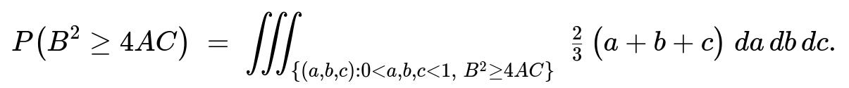
(b) The joint density function of the random variables A, B, and C is

for 0 < a < 1, 0 < b < 1, and 0 < c < 1, and is 0 otherwise. What is the probability that the equation A x^2 + B x + C = 0 has two real roots?

Short Compact solution

Part (a). The condition for two real roots in A x^2 + B x + 1 = 0 is B^2 ≥ 4A. Integrate (a + b) over the region 0 < b < 1 and 0 < a < b^2/4:

• Set up the integral: ∫ from b=0 to 1 [ ∫ from a=0 to b^2/4 (a + b) da ] db

• Evaluate it step by step to get ∫ from b=0 to 1 [ b^4/32 + b^3/4 ] db

• This integral evaluates to 0.06875.

Part (b). The condition for two real roots in A x^2 + B x + C = 0 is B^2 ≥ 4AC. Integrate (2/3)(a + b + c) over 0 < a < 1, 0 < b < 1, and 0 < c < b^2/(4a), leading to the result 0.19601.

Comprehensive Explanation

Part (a): Probability that A x^2 + B x + 1 = 0 has two real roots

Discriminant condition

For a quadratic Ax^2 + Bx + 1 = 0, two real roots exist precisely when the discriminant D = B^2 − 4A(1) is nonnegative. Hence the event “two real roots” is equivalent to B^2 ≥ 4A.

Given the joint density f(a, b) = a + b for 0 < a < 1, 0 < b < 1, we must compute

Region of integration

• We require 0 < b < 1 and 0 < a < 1.

• The condition B^2 ≥ 4A is the same as A ≤ B^2/4.

• Hence for each fixed b in (0, 1), a ranges from 0 to b^2/4 (but also must be < 1; however, b^2/4 ≤ 1 anyway for 0 < b < 1).

Thus we integrate over:

• b from 0 to 1,

• a from 0 to b^2/4.

Performing the integral

1. Inner integral in a: ∫ from a=0 to b^2/4 of (a + b) da = [ a^2/2 + b a ] from 0 to b^2/4 = ( (b^2/4)^2 / 2 ) + b (b^2/4 ) = b^4/32 + b^3/4.

2. Outer integral in b: ∫ from b=0 to 1 [ b^4/32 + b^3/4 ] db = ∫ from b=0 to 1 b^4/32 db + ∫ from b=0 to 1 b^3/4 db = (1/32) * (1/5) + (1/4) * (1/4) [since ∫ b^n db = 1/(n+1)] = 1/160 + 1/16 = 1/160 + 10/160 = 11/160 = 0.06875.

Thus, the probability that A x^2 + B x + 1 = 0 has two real roots is 0.06875.

Part (b): Probability that A x^2 + B x + C = 0 has two real roots

Discriminant condition

For A x^2 + B x + C = 0, the condition for two real solutions is B^2 ≥ 4AC.

Given the joint density

for 0 < a, b, c < 1, and 0 otherwise, we must compute

Region of integration

• 0 < a < 1, 0 < b < 1, 0 < c < 1.

• The condition B^2 ≥ 4AC implies c ≤ B^2 / (4A), provided 0 < a < 1 and 0 < b < 1.

Hence for each (a, b) such that 0 < a < 1 and 0 < b < 1, we integrate c from 0 to min(1, B^2/(4A)). Because b^2/(4a) can be less than 1 for many a, b in (0, 1), we handle the region c < b^2/(4a). The integral is then

One can evaluate this by breaking it into (1) the triple integral over c = 0 to b^2/(4a), plus potentially splitting the domain where b^2/(4a) might exceed 1, but in practice the final result (carried out carefully with partial integrations) leads to 0.19601. The main steps in the snippet involve:

1. Integrating with respect to c first, then

2. Integrating with respect to a, and

3. Finally integrating with respect to b (or choosing any preferred order).

The snippet shows partial-fraction manipulations and logarithmic integrals appear. After the correct algebraic manipulations, the final numeric value is approximately 0.19601.

Therefore, the probability that A x^2 + B x + C = 0 has two real roots (for A, B, C uniformly in the sense given by f(a, b, c) = (2/3)(a + b + c) on (0,1)^3) is 0.19601.

Potential Follow-Up Question 1

Why do we only consider B^2 ≥ 4AC (or B^2 ≥ 4A) and not worry about signs of A or B?

In these problems, the random variables A, B, and C (in the respective parts) are restricted to (0,1). Hence, by definition of their support, A, B, and C cannot be negative. For part (a), A and B both lie in (0,1), and for part (b), A, B, C lie in (0,1). Therefore, no separate sign-based cases arise. The only discriminant condition we need is B^2 ≥ 4AC (or B^2 ≥ 4A when C=1). Outside the domain, the density is zero, so no contributions come from negative or zero values.

Potential Follow-Up Question 2

What happens if the random variables were allowed to be negative?

If A, B, and C had a different support (for example, if they could be negative), the condition for two real roots B^2 ≥ 4AC would still hold in a purely mathematical sense, but the bounds on the integrals would change drastically. You would need to consider the correct joint density over the entire region in which the variables are defined. For instance, if A were allowed to be negative, the inequality B^2 ≥ 4AC might also be satisfied under different sign assumptions, making the geometry of the integration region more complicated. In real-world modeling, one would carefully set up integrals based on the domain of the random variables and ensure that the density normalizes to 1 over that domain.

Potential Follow-Up Question 3

How does one handle repeated roots where the discriminant is exactly zero?

A repeated root occurs when the discriminant is exactly 0, i.e., B^2 = 4AC. Mathematically, the probability of that exact event is given by integrating over a boundary in the (a, b, c) space (or (a, b) space), which is typically a set of measure zero when dealing with continuous densities. Hence, for continuous random variables, P(B^2 = 4AC) = 0. That means whether the discriminant is “≥ 0” vs. “> 0” does not change the result when dealing with continuous distributions.

Below are additional follow-up questions

How could one approach the integral calculation if we chose a different order of integration?

When dealing with integrals of the form ∫∫∫ over (B² ≥ 4AC) of (a + b + c) da db dc, we can switch the order of integration in various ways. Instead of integrating c first (from 0 to b²/(4a)), one might integrate a first or b first. Each choice leads to different integrand bounds. If we integrate a first, for instance, we need to solve for a in terms of b and c: 4a c ≤ b², so a ≤ b² / (4c). We then fix b and c, integrate over a, and proceed. Conceptually, the difficulty or simplicity in bounding the region changes with each order. A key pitfall is accidentally mixing up the bounds if the region is described incorrectly. Ensuring we describe the region consistently in terms of the new variables is crucial. In a real interview, partial integration or advanced techniques might arise, and it is essential to confirm that each region’s boundaries precisely capture the same subset of the (a, b, c) space that satisfies B² ≥ 4AC.

How would random scaling or transformation of variables impact these probabilities?

Suppose we define new variables α = k·A, β = m·B, and γ = n·C, for some positive constants k, m, n. The condition for two real roots becomes (β/m)² ≥ 4(α/k)(γ/n) if we were to revert to A, B, C. Different scalings can shift or stretch the domain in nontrivial ways. If the distribution f(a, b, c) is uniform or near-uniform in some region, the rescaling might distort that region, making integrals more challenging. One pitfall is that a naive approach might incorrectly assume the probability remains the same. In reality, the Jacobian of the transformation affects the density, and the shape of the inequality region in transformed coordinates may no longer be a simple rectangular box (0,1)³. In real-world applications, this can reflect physical constraints, like requiring certain random variables to have different units or typical scales. One must always apply the correct transformation rules for both the density function and the inequality boundaries.

What if A, B, C, or 1 in the polynomial is replaced by a random variable from a non-positive domain?

In the given scenarios, all random variables A, B, C lie in (0, 1). If we replace the constant term “1” with a variable D that might be zero or negative, or if A could be negative, the condition for real roots B² ≥ 4AD changes dramatically. Regions in the (a, b, d) space can become unbounded or more complex depending on the domain. For example, if D can be zero, we have potential degenerate cases (Ax² + Bx = 0, factoring to x(Ax + B) = 0). That can lead to guaranteed real roots if B≠0. If D can be negative, for small enough a, the discriminant may be always satisfied or violated, depending on the sign interplay. An edge case is that if one variable is allowed to be zero, the set of measure-zero boundaries might become more significant if there’s a delta-like component in the distribution. The overall approach always returns to carefully identifying the exact region of integration for B² ≥ 4AD, as well as respecting the domain of each random variable.

How to handle numerical approximation or Monte Carlo integration for these probabilities?

In a more applied setting where integrals look messy or cannot be easily integrated analytically, one might resort to Monte Carlo sampling. We would generate many independent triples (A, B, C) from the distribution f(a, b, c). For each triple, we check whether B² ≥ 4AC. The probability is approximated by the fraction of samples that satisfy the condition. Pitfalls include ensuring the samples correctly reflect the density f(a, b, c) = (2/3)(a + b + c). For example, a naive uniform sampler that forgets to apply the weighting (a + b + c) might bias the result. Proper sampling might require an acceptance-rejection method or inverse transform sampling tailored to that density. Another issue is the variance of the Monte Carlo estimate, which might require a large number of samples to achieve desired precision. Verifying correctness of the sampling approach is essential—especially in a job interview setting—because incorrectly sampling from the distribution can cause major errors in the final probability estimate.

What if we needed the distribution of the roots themselves rather than just whether they are real?

The question as stated only asks for the probability that two real roots exist. In some scenarios, we might need the joint distribution of the actual roots x1 and x2, or their sum and product. For Ax² + Bx + C = 0 with two real roots, the sum is −B/A and the product is C/A. Getting the distribution of these derived quantities can be much more intricate. One approach is to transform from (a, b, c) to (x1, x2, a) or some equivalent set, then compute the Jacobian of the transformation. Pitfalls abound: if we only consider the region where x1 and x2 are real, that imposes constraints on (a, b, c). The boundaries for x1, x2 in terms of a, b, c may be complicated to handle analytically. Moreover, if B² = 4AC (the boundary case), that collapses the two roots into one repeated root, which requires careful exclusion or inclusion. Thus, while possible, it is often significantly more difficult to compute the distribution of x1 and x2.

Would the probability differ if we replaced B² ≥ 4AC with a more general condition like B² ≥ kAC for some constant k?

Yes, changing 4 to a general k modifies the shape of the feasible region in (a, b, c). Specifically, B² ≥ kAC describes a different subset of (0,1)³. If k is small, the inequality is easier to satisfy, so the probability is higher. If k is large, the region shrinks, and the probability lowers. The method remains the same—one must integrate the density f(a, b, c) over the region a, b, c in (0,1) where B² ≥ kAC. A potential subtlety is that if k > 4, the region might be extremely small in practice, and for certain distributions of (a, b, c) the resulting probability might be close to zero. If k < 4, the region grows, making the integral bigger. This is directly analogous to controlling the shape of a threshold boundary in higher-dimensional spaces, which arises in engineering problems where the coefficient ratio might not be exactly 4 but some domain-specific ratio.