ML Interview Q Series: Recurrence Relation for Even Heads Probability in Biased Coin Tosses

Browse all the Probability Interview Questions here.

24. A biased coin with probability p of landing on heads is tossed n times. Write a recurrence relation for the probability that the total number of heads after n tosses is even.

Below is a very detailed exploration of how we can arrive at the correct recurrence relation and all the intricacies that might arise in the process. We will also explore potential follow-up questions that are typically asked in deep technical interviews at major tech companies. Each follow-up question will be presented verbatim in H2 headings, and then we will answer them in exhaustive detail.

Explanation of Core Concepts and Logic

One of the classic ways to handle probability questions involving "number of heads is even" (or odd) after a certain number of coin tosses is to break it down into how parity (even vs. odd) changes with each toss. Let us define:

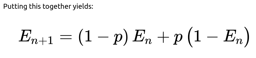
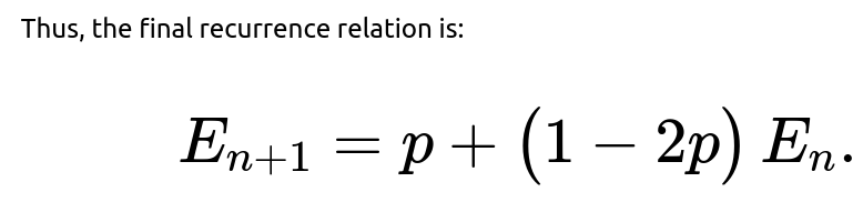
That is the desired recurrence relation for the probability that the total number of heads after n tosses is even.

Implementation Example in Python

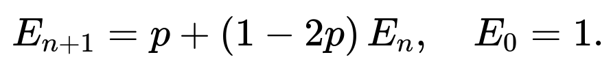
def probability_even_heads(n, p):
    E = 1.0  # E_0 = 1 since with zero tosses, we have 0 heads (which is even)
    for _ in range(n):
        E = p + (1 - 2*p) * E
    return E

# Example usage:
n = 5
p = 0.3
print(probability_even_heads(n, p))  # Probability the number of heads is even after 5 tosses with p=0.3

If there are any tricky follow-up questions, they might look like this:

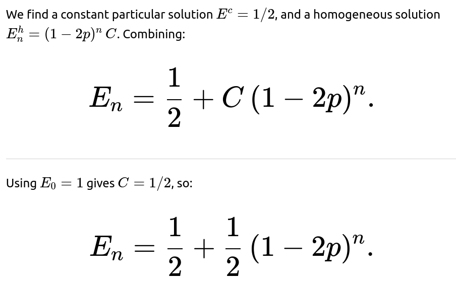
How do we solve the recurrence relation in closed form?

What happens if p=1/2? Why do we get E_n=1/2?

This question often comes up in an interview to ensure the candidate fully understands how special values of p fit into the general formula.

Could we derive a simpler approach if we forget about direct parity reasoning?

In interviews, sometimes the interviewer might probe whether you can solve this problem in other ways. One alternate approach is to let

$$X_i = \begin{cases}

1 & \text{if the } i\text{-th toss is heads},\ 0 & \text{if the } i\text{-th toss is tails}. \end{cases}$$

The important point is that both approaches—parity flipping or direct binomial expansions—lead to the same final expression. In interviews, the simpler explanation of parity flipping from even to odd with probability p often suffices and is quick to convey in a technical setting.

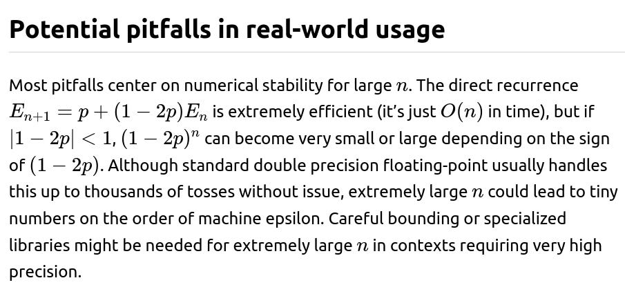
Could floating-point instability be a pitfall in the computation?

This is often a deeper engineering question asked at companies that handle large-scale simulations. It tests your knowledge of implementing math in code reliably under precision constraints.

Is there a more general approach for other moduli?

Summary

The concise, standard recurrence relation that is most often expected in interviews is:

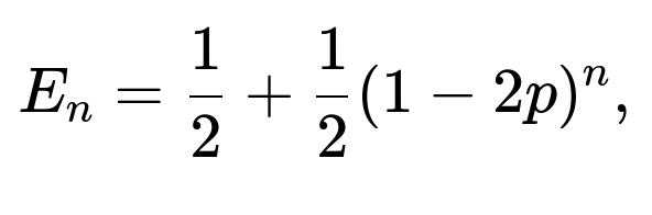
One can either leave the answer in this recurrence form or optionally provide its closed-form solution:

depending on the interviewer’s preference.

Below are some of the common follow-up questions you might encounter on this topic and detailed answers to each.

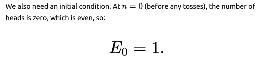
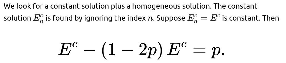
What is the base case for the probability that the total number of heads is even?

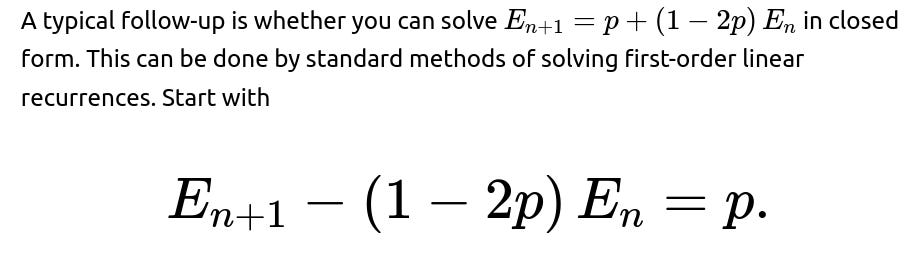
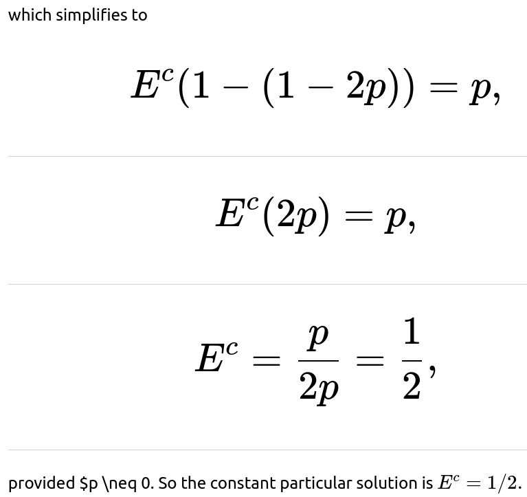
How do you derive and solve the recurrence relation in closed form?

We set up the recurrence as:

Simplifying gives:

We solve by noting it is a first-order linear recurrence:

What if p=1/2?

When p=1/2, the coin is fair. Plugging p=1/2 into the recurrence:

Provide Python code to compute E_n directly from the binomial formula for verification

Though the direct recurrence is more efficient, you might be asked to do a brute force or binomial summation approach for verification. It would look like:

import math
from math import comb

def probability_even_heads_binomial(n, p):
    total_prob = 0.0
    for k in range(n+1):
        if k % 2 == 0:  # check if k is even
            total_prob += comb(n, k) * (p**k) * ((1-p)**(n-k))
    return total_prob

# Example usage:
n_test = 5
p_test = 0.3
print(probability_even_heads_binomial(n_test, p_test))

This code enumerates all k from 0 to n, adds up the probability of k heads, but only when k is even. While this approach is O(n) and can become expensive if n is large, it can be used for small n to confirm the correctness of the recurrence relation. For larger n, the recurrence-based approach is much more efficient.

Conclusion

The key result is that the desired probability satisfies the following recurrence relation:

This is exactly what is typically sought by interviewers when they ask for a "recurrence relation for the probability that the total number of heads after n tosses is even." The most important points are the interpretation of how parity changes with heads or tails and the initial condition. If pushed further, you can present the closed-form solution or code snippets to show how to compute or verify the probability for given n and p.

Below are additional follow-up questions

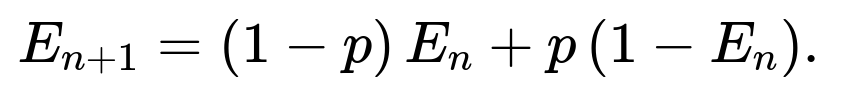
What if the probability of heads changes over time instead of remaining fixed?

When the probability of heads is not constant (i.e., instead of a single fixed value p, we have a sequence of probabilities p₁, p₂, …, pₙ for each toss), we can no longer use the simple recurrence relation Eₙ₊₁ = p + (1 - 2p) Eₙ. That equation critically relies on p being the same on every toss, so that parity flips with probability p and remains the same with probability 1 - p.

To handle a time-varying bias, define Eₙ as the probability that the total number of heads is even after n tosses. For the (n+1)-th toss, which has probability pₙ₊₁ of landing heads, the recurrence modifies to:

Eₙ₊₁ = (1 - pₙ₊₁) Eₙ + pₙ₊₁ (1 - Eₙ).

Here (1 - pₙ₊₁) is the probability of tails on the (n+1)-th toss and pₙ₊₁ is the probability of heads on the (n+1)-th toss. Simplifying:

Eₙ₊₁ = pₙ₊₁ + (1 - 2pₙ₊₁) Eₙ.

Thus, whenever you have a changing probability at each step, you multiply by (1 - 2pₙ) for the homogeneous part for the nth toss. Importantly, you cannot combine all the probabilities into a single expression (1 - 2p)ⁿ any longer; you would need to handle the product or sum iteratively at each step. The base condition remains E₀ = 1. But the final Eₙ would need to be computed step by step if you want an exact value.

Pitfalls include:

• If the probabilities pᵢ vary drastically, you must carefully track each term in the recursion. • Accumulating floating-point errors if n is large and pₙ is near 0.5. Repeated multiplications by (1 - 2pₙ) may cause underflow or precision issues. • The lack of a neat closed-form solution like ½ + ½(1 - 2p)ⁿ. Instead, you have a sequential update.

In real-world applications, time-varying biases might come from non-stationary processes or adaptive systems. Ensuring that code handles these transitions properly is crucial.

How do we extend the approach if the coin tosses are correlated rather than independent?

The recurrence relation we derived fundamentally assumes independence between tosses. If toss i is correlated with toss j, the probability of heads on one toss can depend on previous outcomes. In such a scenario, we can no longer say the parity flips with probability p and remains with probability (1 - p), because the effective probability of heads on toss n+1 might depend on previous results.

One approach is to model the correlation structure explicitly, for example using a Markov chain on pairs of states: "even count so far" and "odd count so far," combined with a correlation parameter that changes how likely the next toss is heads given the previous toss. With correlated coins, you might need a more complex state representation:

• State variables could include both the current parity and the outcome of the last toss if correlation extends only one step back. • If the correlation extends over multiple past tosses, the state space can grow exponentially.

A simple Markov chain extension: Suppose you have two states E (parity so far is even) and O (parity so far is odd). Then you define transition probabilities from E to O and from O to E, but these might depend on the last toss outcome and correlation structure. For example, if we say the probability that the next toss is heads given the previous toss was heads is pₕₕ, and the probability that the next toss is heads given the previous toss was tails is pₜₕ, we end up with a 4-state Markov chain if we also track what the last toss was.

Pitfalls include:

• Handling partial or incomplete correlation structures incorrectly. • Not realizing that the simple recurrence for the unbiased or biased i.i.d. case is invalid once dependence is introduced. • Overcomplicating the system if the correlation extends beyond a one-step Markov assumption.

Real-world scenarios might see correlation when the coin's physical environment changes with each toss or if the coin tosses are not truly random (e.g., a mechanical flaw in how the coin is flicked).

Could we do a moment-generating function or characteristic function approach, and why might it help?

Yes. Instead of directly tracking parity via a recurrence, we can consider the random variable Sₙ = X₁ + X₂ + … + Xₙ, where each Xᵢ is the Bernoulli outcome of the i-th toss. One can use generating functions or characteristic functions:

• Characteristic function of Sₙ: ϕₛₙ(t) = 𝔼[e^(itSₙ)]. • Probability generating function of Sₙ: Gₛₙ(z) = 𝔼[z^(Sₙ)].

For parity, the event Sₙ mod 2 = 0 can be found by evaluating certain sums or by leveraging the identity

𝔼[(-1)^(Sₙ)] = P(Sₙ is even) - P(Sₙ is odd).

Thus,

P(Sₙ is even) = ½ [1 + 𝔼[(-1)^(Sₙ)]].

If the coin is i.i.d. with probability p for heads, then

𝔼[(-1)^(Sₙ)] = ( (1-p) + p(-1) )ⁿ = (1 - 2p)ⁿ.

Hence

P(Sₙ is even) = ½ [1 + (1 - 2p)ⁿ].

This is a more advanced approach that arrives at the same result without explicitly writing the direct parity recurrence. It can sometimes simplify analyzing more complex algebraic manipulations or expansions (like expansions involving cosines if you interpret (-1)^(Sₙ) = e^(iπSₙ)). It’s particularly useful in more general algebraic contexts (e.g., evaluating sums of random variables across moduli).

Pitfalls include:

• Overlooking that (1 - 2p) might be negative; you need absolute values or complex arguments if you extend beyond the simple real domain. • Conflating moment-generating functions (MGFs) with characteristic functions (CFs). In many discrete settings, CFs can be more numerically stable. • If p is close to ½, (1 - 2p) is near 0, so (1 - 2p)ⁿ might underflow quickly for large n. This could cause numerical issues in real implementations.

How can we handle a scenario where we only observe part of the outcomes, or some tosses are missing?

Suppose that out of n planned tosses, some subset is unobserved or lost due to data issues. If you only know that k specific tosses resulted in heads and ℓ specific tosses resulted in tails, while the remaining n - (k + ℓ) tosses are unobserved, you would need a conditional probability approach for parity:

• First, the known heads count might be even or odd. • The unobserved tosses are random Bernoulli(p) draws (assuming i.i.d. and knowledge of p).

Define the random variable U for the number of heads among the unobserved tosses. We are interested in the parity of (known heads + U). If known heads is e (an even number) or o (an odd number), you can compute:

• Probability that U is even or odd using the same formula ½[1 + (1 - 2p)^(n - (k+ℓ)) ].

• Then combine with whether the known heads are even or odd.

For instance, if the known heads count is even, we want U to be even for the total to be even; if the known heads count is odd, we want U to be odd to make the total heads even. This can be done systematically:

• Probability that U is even = Eₘ, where m = n - (k+ℓ). • Probability that U is odd = 1 - Eₘ. • Eₘ can be computed by ½[1 + (1 - 2p)ᵐ].

Hence the final probability is either Eₘ or 1 - Eₘ depending on the known heads’ parity. This approach extends naturally to partial data settings.

Pitfalls include:

• Forgetting to incorporate the known partial outcomes’ effect on parity. • Failing to recalculate if p is not precisely known or must be estimated. • Overlooking that the unobserved tosses might come from a distribution that is not exactly the same p if something changed mid-experiment.

What if we need to compute confidence intervals for the estimated p and how that affects the probability of even heads?

In practical situations, we might not know the coin’s true probability of heads p exactly. We estimate it from data, say from repeated experiments. Then, we might want not just a point estimate for the probability of an even number of heads, but a range that reflects uncertainty in p.

Steps to handle this:

1. Obtain an estimate p̂ from prior tosses or from a different dataset. You might also have a confidence interval for p̂, such as [p̂ₗ, p̂ᵣ] at some confidence level.

2. Recognize that the true p might be anywhere in that interval.

3. For each candidate p in [p̂ₗ, p̂ᵣ], you can compute the probability of even heads, Eₙ(p) = ½ [1 + (1 - 2p)ⁿ].

4. Find the minimum and maximum of Eₙ(p) over p in [p̂ₗ, p̂ᵣ] to get a worst-case or best-case scenario for the probability that heads is even.

It turns out that (1 - 2p)ⁿ is a monotonic function of p if n is fixed. If (1 - 2p) > 0, Eₙ(p) is decreasing in p, and if (1 - 2p) < 0, the function’s sign flips at p=½. Careful analysis of the interval [p̂ₗ, p̂ᵣ] relative to 0.5 is needed to find extremes.

Pitfalls:

• Mixing up frequentist confidence intervals with Bayesian credible intervals and how to interpret them. • If p̂ is extremely close to ½, (1 - 2p) might be near 0, and small changes in p can cause large shifts in (1 - 2p)ⁿ if n is large. That can complicate how quickly the function decays. • Overestimating the precision of p̂ when the sample size is small.

How would you simulate or verify this probability in a large-scale Monte Carlo experiment?

To run a Monte Carlo simulation:

1. Choose p and n.

2. Run a large number of trials, say M. In each trial, simulate n Bernoulli(p) tosses, count how many heads occur, and check if that count is even.

3. Keep track of the fraction of trials in which the count of heads was even.

4. As M → ∞, this fraction should converge to the theoretical probability Eₙ.

For example in Python:

import random

def monte_carlo_even_heads(n, p, M=10_000_000):
    even_count = 0
    for _ in range(M):
        heads_count = sum(random.random() < p for _ in range(n))
        if heads_count % 2 == 0:
            even_count += 1
    return even_count / M

# Example usage:
p_test = 0.3
n_test = 10
approx_prob = monte_carlo_even_heads(n_test, p_test, M=1000000)
print(approx_prob)

Pitfalls:

• For large n, simulating n tosses for each of M trials can be expensive. You might want to rely on the direct formula or recurrence for a more efficient approach. • If p is close to 0 or 1, the distribution of heads is very skewed, which might require a large M to accurately estimate the probability of even heads. • Pseudorandom number generator quality might matter if extremely high precision is desired.

How would we modify the approach if we are summing multiple coins, each with its own probability pᵢ?

Suppose you have coins with probabilities p₁, p₂, …, pₖ, and you toss each coin n times. That’s a total of k·n tosses, but they are grouped or structured differently. If each coin is tossed n times independently from the others, you can sum the total heads from all k coins, which might each have a different probability pᵢ of heads. In general, you have:

Sₙ = Σ (number of heads from coin i in n tosses).

If all tosses are independent across coins:

• Probability that coin i’s count of heads is even after n tosses can be found by the same formula ½ [1 + (1 - 2pᵢ)ⁿ]. • However, to find the probability that the total sum Sₙ is even, you cannot simply multiply or add these probabilities, because whether coin i’s heads count is even or odd also depends on coin j’s. You need to track the combined parity.

A more direct approach is to define Eᵢ(n) = Probability that coin i has an even number of heads in n tosses. Then consider the random variables individually:

• Let Yᵢ be an indicator that coin i’s heads count is even. Then the parity of Sₙ is even if the sum of Yᵢ across all i for which the coin’s heads count is odd is itself even. That can get complicated quickly.

Another approach is to note that for each coin i:

P(Sₙ is even) = ½ [1 + 𝔼[(-1)^(Sₙ)]].

But Sₙ = Σ (Xᵢ,ⱼ), where Xᵢ,ⱼ is the j-th toss outcome of coin i. Then

𝔼[(-1)^(Sₙ)] = 𝔼[Πᵢ,ⱼ (-1)^(Xᵢ,ⱼ)] = Πᵢ,ⱼ 𝔼[(-1)^(Xᵢ,ⱼ)],

assuming independence across all coins and tosses. For each Xᵢ,ⱼ with probability pᵢ of being heads,

𝔼[(-1)^(Xᵢ,ⱼ)] = (1-pᵢ) · 1 + pᵢ · (-1) = 1 - 2pᵢ.

So each coin tossed n times contributes (1 - 2pᵢ)ⁿ. Hence:

𝔼[(-1)^(Sₙ)] = Πᵢ (1 - 2pᵢ)ⁿ.

Therefore:

P(Sₙ is even) = ½ [1 + Πᵢ (1 - 2pᵢ)ⁿ].

Pitfalls:

• Forgetting to handle the fact that each coin can have a different pᵢ. • If some pᵢ = ½, then (1 - 2pᵢ) = 0, forcing that product to be 0, which typically yields P(Sₙ is even) = ½. • Overcomplicating the state space if you try to track individual parities. The generating function approach (or characteristic function approach) is usually simpler here.

How do we compute the variance or higher moments of the indicator of “even number of heads”?

Define the indicator random variable Iₙ = 1 if Sₙ is even, and 0 if Sₙ is odd. We already know 𝔼[Iₙ] = P(Sₙ is even). For a typical i.i.d. scenario with probability p:

𝔼[Iₙ] = Eₙ = ½ [1 + (1 - 2p)ⁿ].

If you want Var(Iₙ), recall Var(Iₙ) = 𝔼[Iₙ²] - 𝔼[Iₙ]². Since Iₙ is an indicator, Iₙ² = Iₙ, so 𝔼[Iₙ²] = 𝔼[Iₙ] = Eₙ. Hence:

Var(Iₙ) = Eₙ - Eₙ² = Eₙ(1 - Eₙ).

Therefore:

Var(Iₙ) = ½ [1 + (1 - 2p)ⁿ] · ½ [1 - (1 - 2p)ⁿ].

We can simplify:

= ¼ [1 - (1 - 2p)²ⁿ].

This follows because (1 + x)(1 - x) = 1 - x². So:

Var(Iₙ) = ¼ [1 - (1 - 2p)²ⁿ].

Pitfalls:

• Confusing the variance of Iₙ with the variance of the total heads Sₙ. They are very different. • Overlooking that the indicator variable can only take values 0 or 1, so it has a simpler formula for variance than a general random variable. • Not applying 𝔼[Iₙ²] = 𝔼[Iₙ], which is a standard property of indicators.

What happens if we are asked for the probability that the number of heads is odd, and is there a direct recurrence?

The probability that the number of heads is odd after n tosses is simply 1 - Eₙ, where Eₙ is the probability of even heads. For an i.i.d. coin with probability p of heads:

P(Sₙ is odd) = 1 - ½ [1 + (1 - 2p)ⁿ] = ½ [1 - (1 - 2p)ⁿ].

If you’d like a direct recurrence, define Oₙ = P(Sₙ is odd). Then from a parity-flip perspective:

• If it was odd before (Oₙ), it remains odd with probability 1 - p (we get tails), and flips to even with probability p (heads). • If it was even before (Eₙ), it flips to odd with probability p and stays even with probability 1 - p.

So:

Oₙ₊₁ = (1 - p)Oₙ + pEₙ.

Since Eₙ + Oₙ = 1, you can rewrite Oₙ₊₁ in a similar form:

Oₙ₊₁ = p + (1 - 2p)Oₙ.

The same base condition logic applies: O₀ = 0 (because with zero tosses, we have zero heads, which is even). Indeed, everything lines up with Oₙ = ½ [1 - (1 - 2p)ⁿ].

Pitfalls:

• Missing that O₀ = 0 is different from E₀ = 1. • Not noticing that Oₙ = 1 - Eₙ is all you need if Eₙ is known. • Accidental sign mistakes in expansions.

How would we address partial or total ordering constraints on the heads?

Sometimes, an interviewer might twist the question: “What if you only count the number of heads among tosses that occur after the first tail?” or “What if you skip the first H heads?” Then you cannot directly apply the same even-odd analysis without adjusting how you define the random variable that tracks heads. You must carefully define your random process:

• For example, if you wait until the first tail occurs, only then do you start counting heads for parity. That effectively means your random variable’s domain depends on a stopping time (the time you see the first tail). • This can be turned into a new random variable problem: define T as the index of the first tail. Condition on T and then count the heads that follow T.

Each such twist can drastically alter the distribution. You often must set up a conditional probability or handle geometric random variables for the waiting times, then do a parity analysis on the post-tail tosses. The key to success is rewriting the problem carefully in terms of well-understood random variables. Then you can attempt to either create or adapt the known parity recurrences.

Pitfalls:

• Incorrectly applying the i.i.d. assumption to a random number of tosses if you’re dealing with a stopping time. • Overlooking that the number of tosses might be random, changing the probability space. • Getting the boundary conditions wrong if T can be 1 or if T can be up to n, etc.

Could we use the concept of a reflection principle or combinatorial argument to prove the even-odd probability?

In certain combinatorial or gambler’s ruin scenarios, a reflection principle is used to map paths with a certain property to paths with a complementary property. While typically the reflection principle is used for random walks crossing boundaries, you can sometimes adapt these arguments to count how many sequences of coin tosses lead to an even number of heads vs. an odd number. The reflection principle approach might go:

1. The total number of sequences of length n is 2ⁿ.

2. The difference between the number of sequences with an even number of heads and those with an odd number of heads can often be found by applying a certain involution or reflection that pairs sequences with opposite parity.

3. One can show that the difference is ( (1-p) - p )ⁿ = (1 - 2p)ⁿ after weighting each sequence by its probability.

The direct reflection argument is more standard for a fair coin (p=½), in which case it’s easy to pair each sequence with exactly one that flips the outcome of the first toss. For a biased coin, the principle is more subtle but can still be applied using weighted or sign-based enumerations.

Pitfalls:

• Failing to account for weighting by p when counting sequences. A pure combinatorial reflection principle for p=½ might not directly carry over without adjusting for the bias factor. • Overcounting or double-counting sequences if not careful with how the reflection is defined. • Attempting to apply a naive combinatorial argument that only works in the unbiased case to the biased scenario incorrectly.

How to handle random stopping times, such as “stop tossing once we have r heads” and then check parity?

In some problems, you stop tossing the coin once you have r heads in total, or once you have r tails, or something else. The number of tosses N is itself random. Then you might ask: “What is the probability that the total number of heads at stopping time N is even?” But if we always stop once we have r heads, then obviously the final count of heads is r (which might be even or odd deterministically). So that question might be trivial.

But if we define something else, like “stop once we have r heads or s tails, whichever happens first,” then the final number of heads might be r or anything less than that if s tails occurred first. The analysis then uses gambler’s ruin or negative binomial style distributions. The parity question becomes more intricate:

1. Let N be a stopping time determined by some criterion involving heads and tails.

2. The distribution of N can be complicated (e.g., a negative binomial distribution if you stop upon achieving r heads).

3. We must figure out the parity of the final heads count, which may be r (if we reached r heads first) or some other value if we reached s tails first.

4. Each scenario typically requires a state-based or Markov chain approach with states denoting (current heads count, current tails count), continuing until one dimension hits its threshold. Then we check whether the final heads count is even or odd.

Pitfalls:

• A naive attempt to keep the same recurrence Eₙ₊₁ = p + (1 - 2p) Eₙ fails if n is not fixed but random. • Overlooking that we might want 𝔼[I(N)], where I(N) is an indicator that the final count is even, but the distribution of N depends on r, s, and p. • If r is always the stopping criterion for heads, the question might trivially yield 0 or 1 for certain parities of r. If r is even, the probability is 1. If r is odd, the probability is 0—assuming we definitely stop at r heads eventually.

What if we want to track the probability that the total number of heads is even or odd at every single toss from 1 to n?

In some interview scenarios, you might be asked to produce a sequence E₁, E₂, …, Eₙ, or O₁, O₂, …, Oₙ, describing the probability of even (or odd) heads after each toss. You can easily do this iteratively with the original recurrence:

• E₀ = 1. Then for each j in 0..(n-1):

Eⱼ₊₁ = (1 - p) Eⱼ + p (1 - Eⱼ).

Which simplifies to:

Eⱼ₊₁ = p + (1 - 2p) Eⱼ.

• After j steps, you’ll have Eⱼ for j = 1..n.

Pitfalls:

• Not initializing E₀ = 1. If you start at E₁ incorrectly, you might offset the entire sequence. • If you do an on-the-fly simulation or partial updating in code, watch out for index mixing or off-by-one errors. • Failing to note that from a certain point onward, if p=½, Eⱼ = ½ for all j ≥ 1. That might help optimize or short-circuit computations if you know n is large.

How could we incorporate advanced variance reduction techniques if performing a simulation?

If you decide to estimate P(Sₙ is even) via simulation (maybe p is complicated, or the tosses are correlated in a certain way), variance reduction techniques can speed up the convergence of your estimate:

• Antithetic variates: For each simulated sequence of tosses, create a complementary sequence that flips heads to tails and tails to heads. This can help reduce variance if used properly with an unbiased coin. With a biased coin, you still can attempt a weighting strategy, though it’s more complicated. • Control variates: If you can easily compute an approximate or partial result analytically, you can use that partial result to reduce the variance of the simulation estimate. • Stratified sampling: If you want to ensure coverage of different numbers of heads, you might purposely sample a fraction of paths with a certain distribution to reduce variance.

Pitfalls:

• Implementing antithetic sampling incorrectly for a biased coin. The effect might not be symmetrical, so you have to be sure the approach remains unbiased. • Overlooking the correlation introduced by advanced variance reduction approaches. • Using large memory to store pairs or stratified subsets in an extremely high-dimensional scenario (if n is large).

How might the probability of even heads factor into a hypothesis testing problem?

Consider a scenario: “If the coin is fair, the probability of an even number of heads after n tosses is exactly ½. Observing an even count or odd count might inform you about potential bias if you repeat the experiment many times.” Possibly, the interviewer wants you to interpret the count’s parity across repeated experiments as a data point to test H₀: p = ½ vs. H₁: p ≠ ½. However, parity alone is a single bit of information from each set of n tosses, so it might not be as powerful as using the full count or a more standard binomial test. But you can still analyze how often you get even vs. odd in repeated runs:

• Under H₀, P(Sₙ is even) = 0.5. So in multiple experiments, about half the time you should see even heads, half odd. • Under H₁: p ≠ 0.5, P(Sₙ is even) = ½ [1 + (1 - 2p)ⁿ], which is not 0.5 if p ≠ 0.5. Observing the empirical frequency of even heads across repeated experiments might be used in a test statistic.

Pitfalls:

• Not realizing that you lose a lot of information by only observing the parity and ignoring the magnitude of the head count. The classical binomial test is more powerful. • If p is close to ½, it requires many repeated experiments to detect a significant deviation from 0.5 in the parity frequency. • If n is large, (1 - 2p)ⁿ might be very close to 0 for moderate p ≠ ½, making the probability of even heads approach ½ quickly, reducing detectability.

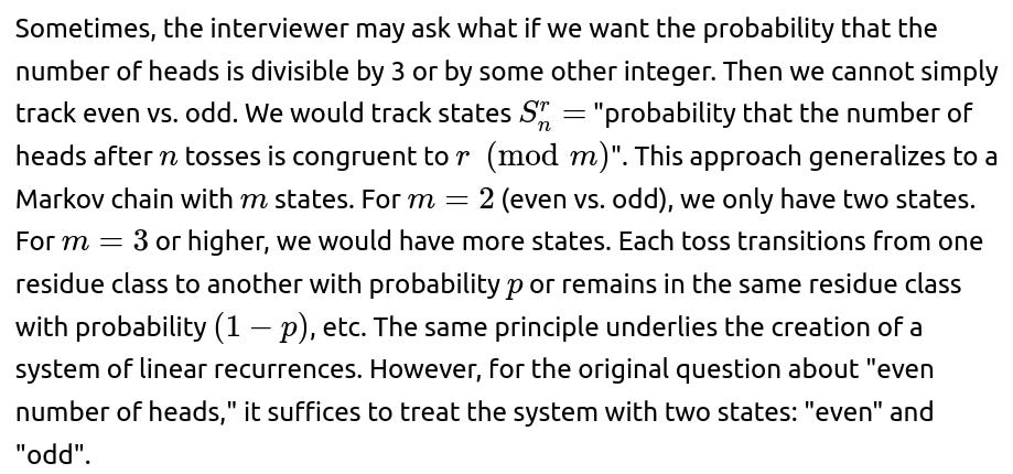
How could the “even heads” concept generalize to higher moduli, such as “the number of heads mod m = k”?

For moduli m > 2, the straightforward approach is to track the probabilities of each residue class modulo m. Define Pₙ(r) = Probability(Sₙ ≡ r (mod m)). Then, for each toss, the distribution over residue classes transitions according to the probability p of heads and 1-p of tails, but you shift from r to (r+1) mod m if a head occurs, or remain in r if a tail occurs (plus do it for all r with the right weighting). Concretely:

Pₙ₊₁(r) = p · Pₙ((r-1) mod m) + (1 - p) · Pₙ(r).

For the even-odd case, m=2, so you only have two states: 0 (even), 1 (odd). For general m, you have m states, leading to a linear recurrence of length m. It can be solved using matrix exponentiation or iterative updates. A closed form might be more involved for general m.

Pitfalls:

• Overlooking the difference between a two-state system and an m-state system. The latter is more complex and may not yield to a simple formula like (1 - 2p)ⁿ. • Not implementing the (r-1) mod m index carefully, resulting in an off-by-one or negative index bug in code. • For large n, direct iteration can be slow, but matrix exponentiation can reduce it to O(m³ log n). This is a more advanced approach often tested in algorithmic interviews.

What if we measure the difference in probabilities for even vs. odd heads rather than the probability itself?

Define Δₙ = P(Sₙ is even) - P(Sₙ is odd). Obviously, Δₙ = 2P(Sₙ is even) - 1 = (1 - 2p)ⁿ for an i.i.d. coin. Then P(Sₙ is even) = (1 + Δₙ)/2. Some interviewers might ask to track that difference. The update step for Δₙ from Δₙ₋₁ is:

Δₙ = ( (1-p) - p ) · Δₙ₋₁ = (1 - 2p) Δₙ₋₁.

Hence Δₙ = (1 - 2p)ⁿ. This representation can be convenient in certain proofs or code.

Pitfalls:

• Forgetting to interpret negative values of (1 - 2p)ⁿ. If p > ½, (1 - 2p) is negative, so Δₙ might alternate in sign for odd/even n. • Confusing Δₙ with P(Sₙ is even) itself. • Not verifying that if Δ₀ = 1 (since at n=0, P(even)=1, P(odd)=0), then indeed Δ₀=1 as well, so everything lines up with Δₙ = (1 - 2p)ⁿ.

How do we handle large n where (1 - 2p)ⁿ underflows in floating-point arithmetic?

If n is extremely large and p is not extremely close to ½, (1 - 2p)ⁿ can quickly become very small (or large if p < ½ but in absolute value it might become small if (1 - 2p) is between -1 and 1). If, for instance, p = 0.4, then (1 - 2p) = 0.2, and 0.2ⁿ can underflow to 0.0 in double precision for large n. This can lead to P(Sₙ is even) being computed as ½ [1 + 0] = ½ even if the true value is slightly above ½. Usually, for large n, that approximation is effectively correct if (1 - 2p)ⁿ is smaller than machine epsilon (~10⁻¹⁶ in double precision).

If you need more precise or symbolic results for intermediate n or for p extremely close to ½:

• You can use higher-precision arithmetic libraries such as Python’s decimal or fractions modules. • You can store the log of |(1 - 2p)ⁿ| = n ln|1 - 2p| and keep track of the sign to reconstruct (1 - 2p)ⁿ without direct exponentiation in floating point. • If p is exactly ½, (1 - 2p) = 0, so it’s trivial that for n ≥ 1, P(Sₙ is even) = ½.

Pitfalls:

• Unexpectedly flipping the sign of (1 - 2p)ⁿ if p > ½; you must keep track of whether n is odd or even. • Inadvertently losing all precision, leading to a naive conclusion that P(Sₙ is even) = ½ for large n. While that might be correct in a practical sense, if extremely high precision is required, you might need special handling. • Overlooking that some systems or languages automatically clamp to 0 for extremely small floating-point exponents, so you get numeric 0 earlier than expected.

How could we incorporate partial knowledge about the coin’s physical properties into the model?

In real-world conditions, a coin’s bias might come from physical asymmetry, spinning technique, or environment. If you have partial knowledge, such as “the coin is heavily weighted toward heads” but not an exact p, you might use a prior distribution over p. Then:

• Bayesian approach: You start with a prior distribution over p, say Beta(α, β). After observing tosses, you update the posterior Beta(α + number_of_heads, β + number_of_tails). • You can then compute the posterior predictive distribution for new tosses or the posterior distribution of the parity probability itself: P(Sₙ is even | data).

This typically involves integrating the expression for P(Sₙ is even | p) = ½ [1 + (1 - 2p)ⁿ] over the posterior distribution of p. The integral might not always have a closed form, so you might do a numeric approximation:

• P(Sₙ is even | data) = ∫ ½ [1 + (1 - 2p)ⁿ] f(p | data) dp.

Pitfalls:

• Confusing frequentist and Bayesian interpretations. • The integral over (1 - 2p)ⁿ might have complexities or require numerical approximation if α + β is large. • If the coin is extremely biased, (1 - 2p) might be large in magnitude (possibly negative if p>½), requiring careful sign handling for big n.

How to design an efficient data structure for streaming coin tosses to track even parity in real time?

If coin tosses arrive in a data stream and we want to know at any time if the total heads so far is even or odd, we can maintain a streaming parity bit:

• Start with a parity variable (initially 0 for “even,” 1 for “odd,” or vice versa). • Each time we observe a head, flip the parity bit; each time we observe a tail, leave it as is.

In code:

parity = 0  # 0 for even, 1 for odd
while True:
    toss = get_next_toss()  # heads=1 or tails=0
    if toss == 1:  # heads
        parity = 1 - parity
    # Now parity indicates if total heads so far is even or odd

However, in a setting where the coin is biased, you might also want to keep track of how many tosses have occurred to compute the probability of being in the even state vs. the odd state. If you only track the parity bit, you know whether the realized outcome so far is even or odd. But you lose direct knowledge about the probability distribution if you want to do more advanced queries like “What if we had not observed some partial toss?”

Pitfalls:

• Relying solely on the single parity bit means you cannot do statistical inference about p without the full count or a running count of heads. • If some toss results are missing or uncertain, you can’t properly update the parity. • If the coin’s bias is unknown, you also need data to estimate p.

How could parity checks help in error detection or coding theory?

Though tangential to the direct probability question, interviewers might mention that the concept of “even parity” is used in error-detecting codes (e.g., a single parity bit appended to a message). The principle is the same: you track whether the sum of bits is even or odd. In coding theory:

• The chance of undetected single-bit error is minimized if you use parity bits to ensure the total sum is even (or odd). • If the parity bit doesn’t match the actual sum of the data bits mod 2, we know an error occurred (at least one bit flipped).

But if the error flips two bits, you may not detect it with a single parity bit. This has some analogy with the “probability that an error remains undetected” in a random error model. One can do a more advanced analysis if the error probability is p for each bit, and you want to know the probability that an even number of errors happen so that the parity check fails to detect them. This becomes essentially the same formula for the probability of an even number of Bernoulli(p) events.

Pitfalls:

• Misinterpreting how an even parity scheme fails to detect an even number of bit flips. • Overlooking that coding theory can add multiple parity bits across different subsets of bits, which complicates the “probability that an error is detected” formula. • Failing to connect that the underlying math is identical to the probability of having an even number of heads in n Bernoulli draws, but now they are bit flips in a message.

How might the probability of even heads appear in quantum computing or physics contexts?

In quantum settings, measuring the parity of a set of qubits might be relevant. The mathematics can mirror the classical parity question, but with amplitudes and interference rather than classical probabilities. For instance:

• A state might be a superposition of basis states that correspond to different counts of “1” qubits. The measurement outcome “even parity” might have a probability amplitude that is the sum of amplitudes for basis states with an even number of 1s. • In classical limit or measurement terms, you can see parallels to the classical probability scenario, especially if the measurement outcomes are effectively random with some distribution.

Pitfalls:

• Confusing quantum amplitude-based analysis with classical probability. • Over-simplifying a quantum superposition to a classical Bernoulli distribution. • Failing to notice that quantum entanglement can create correlations that do not obey the i.i.d. assumption.

How can you handle multi-dimensional parity checks, for instance if we have multiple categories instead of just heads/tails?

In advanced data analysis, you might have multiple categories per trial, e.g., if you roll a die. The concept of “even heads” could generalize to “even occurrences of category X.” That portion remains the same if category X is a single event that occurs with probability p. But if multiple categories are being tracked simultaneously (like “number of times we get category 1 mod 2, category 2 mod 2, etc.”), you might track a vector parity. The update rules become:

• Each trial increments exactly one coordinate in the categorical vector. • You track parity for each coordinate.

This yields a 2ᵏ-state machine if there are k categories for which you track parity. The complexity grows rapidly. A typical approach is to define a generating function in multiple variables, or a 2ᵏ × 2ᵏ state transition matrix, to track how parities evolve. The simpler the question (like “just the parity of heads vs. not-heads” in a coin), the simpler the recurrence.

Pitfalls:

• Not scaling the approach well if the number of categories is large. • Attempting to store the entire distribution of parities across categories in a naive manner. • Failing to realize that if each category’s event probability is small, you might approximate or compress states.

How does knowledge of such a simple recurrence help in understanding more general binomial or distribution problems?

Understanding how parity emerges from sums of Bernoulli variables is a microcosm of how linear recurrences, generating functions, and combinatorial identities can be used to derive closed-form probabilities for events in distribution problems. Specifically:

• The concept of parity flipping with each head vs. staying the same with each tail is an example of a two-state Markov chain, which is the simplest type of chain. Many more complex problems reduce to a chain with more states or transitions. • The direct sum approach using generating functions or characteristic functions is a broader technique: 𝔼[z^(X₁ + X₂ + … + Xₙ)] = Πᵢ 𝔼[z^(Xᵢ)] if the Xᵢ are independent. This can lead to neat closed forms for events that can be described by exponents of z or -1. • Interviewers may probe your knowledge of such simpler recurrences as a stepping stone to more complicated dynamic programming or Markov chain solutions.

Pitfalls:

• Sticking solely to the parity example and missing the bigger picture of using states and transitions for general distribution events. • Not realizing that the principle behind “flip with probability p, remain with probability 1-p” is the foundation of many discrete-time Markov processes. • Overlooking that the same approach can apply if you track the sum modulo some integer m or other transformations.