
ML Interview Q Series: Regression to the Mean: Why Credit Model Cutoffs Overestimate Actual Creditworthiness
📚 Browse the full ML Interview series here.
Assume we have some credit model, which has accurately calibrated (up to some error) score of how credit-worthy any individual person is. For example, if the model’s estimate is 92% then we can assume the actual score is between 91 and 93. If we take 92 as a score cutoff and deem everyone above that score as credit-worthy, are we over-estimating or underestimating the actual population’s credit score?
This problem was asked by Affirm.
When we define a cutoff at the model’s point estimate (in this case 92) and use it to classify individuals as “credit-worthy” or “not credit-worthy,” we will typically end up overestimating the true average credit score of those classified as “credit-worthy.” The reason is tied to the notion of regression to the mean and how uncertainty in the model’s estimates influences outcomes.
In more detail, whenever we see an estimate that is high (e.g., near or above 92), the true score has some probability of being lower (due to noise and imperfect estimates). Because we choose only those individuals whose estimated scores are above this threshold, our chosen subset’s actual scores tend to be somewhat lower on average than their estimated scores. Effectively, by picking any individual with an estimate above 92, we are including cases where their true scores might lie below 92 (as long as the model’s estimation error pushed them above the cutoff). Hence, across the entire subset, the true average credit score is apt to be somewhat lower than 92, meaning we overestimate the population’s credit score with this threshold-based rule.
Below are deeper explanations and follow-up questions that might be asked in a rigorous interview scenario, each addressed carefully and in detail.
Why does regression to the mean cause an overestimation?
One way to frame the effect is through conditional expectations. If a model’s score S is an estimate of a true credit score T, and there is some noise ε, then we can write (in a simplified form):
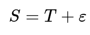
with ε representing random estimation error (which we generally assume to have zero mean and some variance). When we only look at those individuals for whom the estimate S exceeds 92, we are examining E[T∣S>92]. Because S>92 can occur either by T truly being above 92 or by noise fluctuations that push a lower true score above 92, the expected actual score within that group is typically a bit lower than the average of their estimated scores. This is the classic “regression to the mean” phenomenon: extreme observed values (here, “extreme” means above a certain cutoff) are often partly driven by noise, and thus the conditional true value given the observed extreme is less extreme.
Hence, when we say “If the model’s estimate is 92%, we can assume the actual is between 91% and 93%,” that interval reflects an individual’s underlying uncertainty. Once we pick individuals whose estimates exceed 92, the actual average among that group is typically going to drop slightly below 92 in expectation. So, we end up with an overestimation if we assume their true average must also exceed 92.
How does calibration interact with overestimation?

Being “accurately calibrated” implies that, if you take all individuals with model-predicted scores of 92, their average true score is indeed around 92. But once you apply a threshold—particularly a strict one like “above or equal to 92”—you shift the population to one where some fraction of them might have had a slightly inflated estimate due to noise.
Could we ever be underestimating the actual population’s credit score?
It is theoretically possible to underestimate in small edge cases—for instance, if the model is systematically conservative near the boundary of 92. But for a broad population, especially if the errors are roughly centered around zero, the phenomenon of regression to the mean tends to dominate in a threshold-based selection. Consequently, in most real-world applications, you end up overestimating the group’s true mean if you judge them solely by their model-based threshold crossing.
How might we adjust our selection strategy to reduce this overestimation?
One typical approach is to incorporate the distribution of uncertainty around each individual’s estimate. Instead of a hard cutoff of 92, one might:
Use an expected value estimate conditioned on crossing that boundary. In effect, if you see a point estimate of 92, you might discount it slightly (knowing that regression to the mean will pull it down). Tools such as Bayesian adjustment can help address this by “shrinking” extreme values toward the mean of the prior distribution.
Alternatively, one can broaden the acceptance band for borderline cases, thereby reducing the strictness of the threshold and alleviating some of the selection bias.
Could this create real-world fairness or regulatory concerns?
Yes. Credit decisions often fall under strict regulatory oversight. Overestimation might lead to an apparent belief that you are giving loans to only high-scoring individuals, even though some are actually less creditworthy in truth. If the model’s error correlates with protected attributes (e.g., demographic factors), it might disproportionately misclassify or lead to unintended biases. Ensuring that the threshold-based selection does not introduce harmful biases is critical. Model documentation, fairness audits, and periodic recalibration or model retraining can help address these issues.
How do we measure whether our model is overestimating or underestimating in practice?
In practical machine learning pipelines, we typically have a portion of the data set aside for validation or backtesting. We can:
Compare predicted scores vs. actual outcomes to see if threshold-based selection leads to a mismatch. For example, we might measure the average actual outcome for those whose estimated score was above 92 and see if it truly matches or falls below that 92 threshold in reality.
Plot reliability diagrams and calibration curves. If we see that predictions above a certain level do not match the observed fraction, that suggests a calibration or thresholding bias.
Use uplift-based or net benefit-based metrics. Sometimes business metrics (like default rates or net revenue) are used to measure whether choosing the threshold at 92 is capturing the correct portion of creditworthy individuals.
Could a different error distribution change the conclusion?
If the distribution of estimation errors is strongly asymmetric, or if the model systematically overestimates or underestimates at particular score ranges, then the effect could change. However, in practice, most standard modeling assumptions (e.g., that errors around an estimate have a mean of zero and some bounded variance) lead to a result where, once you condition on crossing a threshold, the true mean is pulled back. That is the typical situation in real-world credit models, resulting in an overestimation of the actual group average.
How might we mitigate selection bias in code?
Below is a sketch of how one might empirically test and mitigate threshold-based bias in Python. This is a simplified illustration, but it helps clarify how data scientists might detect and partially correct for overestimation in practice.
import numpy as np
import pandas as pd

# Suppose we have data: actual_scores and model_estimates
# Both are arrays or columns in a DataFrame, each person's actual true credit score and the model's estimate
np.random.seed(42)

# Synthetic example
actual_scores = np.random.normal(loc=92, scale=1.0, size=10000)
model_estimates = actual_scores + np.random.normal(loc=0, scale=1.0, size=10000)

# We'll set a cutoff
cutoff = 92
selected_indices = model_estimates >= cutoff
selected_estimates = model_estimates[selected_indices]
selected_actuals = actual_scores[selected_indices]

print("Mean of model estimates for selected group:", np.mean(selected_estimates))
print("Mean of actual scores for selected group:", np.mean(selected_actuals))

# We might attempt a simple correction by subtracting an average known bias
# from the selected model estimates. For demonstration, let's say we discovered
# an average bias of 0.5
bias_correction = 0.5
corrected_estimates = selected_estimates - bias_correction
print("Mean of corrected estimates for selected group:", np.mean(corrected_estimates))
In a real situation, you would determine any systematic bias from historical holdout sets or carefully calibrated data. By examining the mean of selected_actuals, you would see how it differs from the mean of selected_estimates and then adjust accordingly.
How would you explain this phenomenon to non-technical stakeholders?
In non-technical terms, you might say: “We filter on a particular cutoff that comes from the model. But because the model isn’t perfect, some people whose true credit score is below our cutoff sneak in (the model’s noise inflated their score), while others who are truly above the cutoff might be excluded (the model’s noise deflated their score). On balance, those we do include end up having an actual average creditworthiness slightly below what the model predicts—so if we rely naively on the cutoff score to estimate the group’s true average, we’re overshooting.”
How do we ensure our threshold decision is optimal for the business context?
Choosing the cutoff in credit decisions usually considers:
Expected default rates and profit/loss calculations. A small difference in the actual average creditworthiness of an accepted group can significantly alter net profitability or default risk.
Cost of misclassification. Approving someone with a genuine score below the threshold might be more costly than rejecting someone whose true score is just above it—this can vary by organization.
Strategic acceptance rates. Affirm, for instance, might try to maximize acceptance rates while keeping default risk low enough to remain profitable. The final threshold is often selected via cost–benefit trade-off analysis, not purely from the predicted score.
Could the distribution of scores shift over time?
Yes, and that is a key concern. If population or economic conditions change—say, there is a recession—then the underlying distribution of true credit scores might shift downward (or upward after an economic boom). Even with a well-calibrated model at training time, you may see drift, and your threshold (e.g., 92) might become out-of-date. This real-world drift is why recalibration or continuous retraining is essential.
Summary of the Main Answer
By setting the model’s estimated cutoff at 92 and defining “credit-worthy” as anyone above that estimated value, we are typically overestimating the group’s true creditworthiness. This arises due to regression to the mean: those who squeak over the threshold partly do so due to random noise, so their actual average tends to be lower than the model’s point estimate.
Below are various deeper follow-up questions an interviewer might ask, each clarified for thorough understanding.
Are there specific model types or algorithms where this phenomenon is more pronounced?
Yes. The effect of overestimation given a hard cutoff is fairly universal whenever you have noisy estimates. However, certain models (like large ensemble methods or neural networks) might exhibit heteroskedastic errors: in some regions of the input space, the model is more uncertain than in others. If the region near 92 happens to be one with larger error variance, you might see an even stronger mismatch. Conversely, if the model’s confidence intervals are tighter around 92, the effect might be somewhat smaller but seldom disappears entirely.
Could ensemble averaging reduce the overestimation?
Ensemble averaging (e.g., combining multiple models) can reduce the variance of the estimation error. That can reduce but not necessarily eliminate the selection bias from a threshold-based approach. In practice, ensembles produce more stable (less noisy) estimates, which can mitigate but not fully remove the fundamental phenomenon that conditioning on an extreme (or boundary) subset still pulls in some portion of the population whose true scores are below that boundary.
If the model says “92% ±1%,” how does that ±1% get estimated?
That ±1% can come from techniques such as:
Analytical approximations (e.g., from logistic regression variance–covariance matrices). Bootstrapping or cross-validation, where we measure how much the predicted score fluctuates based on resampled training data. Bayesian posterior intervals, if the model is formulated with distributions over parameters.
Regardless of how the interval is estimated, the selection bias problem remains if we classify based on a single snapshot estimate and ignore the uncertainty bounds.
Could we handle borderline candidates with a “gray zone” instead of a single cutoff?
A gray zone approach (sometimes used in medical diagnosis) is where, instead of a single cutoff, you define a small range around it—for example, 91 to 93—where you request additional information or run further analysis. Individuals whose estimates fall outside this band are straightforward accept/reject decisions, while those in the band get deeper review or require additional features. This strategy:
Reduces the number of borderline cases that might be mislabeled due to noise. Incorporates a second decision layer, which can incorporate more data or a stricter check.
Practical tips for an interview scenario
Explain that purely because of random noise, the “above 92” group’s true average will be closer to the overall average, not the extreme high. Hence you are “overestimating” if you assume the group’s actual average is 92 or higher. Mention that well-calibrated models still exhibit this phenomenon due to sampling and noise. Highlight that real-world solutions often involve some combination of adjusting for known biases, including well-thought-out acceptance rates, or adopting more robust decision frameworks.
Conclusion
In conclusion, taking 92% as a strict cutoff and deeming everyone above that score to be credit-worthy generally overestimates the group’s actual credit scores. This stems from regression to the mean, calibration nuances, and the inherent noise in model predictions. Even perfectly calibrated models exhibit this effect once we condition on crossing a specific threshold. Adjusting decision boundaries, using “gray zones,” or accounting for the conditional expectation can help mitigate the discrepancy and ensure the threshold aligns with actual credit risk.
How does this logic extend beyond credit scores?
This phenomenon applies to many domains where a noisy estimate is thresholded to select the top performers or best prospects—hiring decisions, lead scoring, or even medical tests. Whenever you rely on point estimates plus a cutoff, you risk seeing the true mean of that selected group end up lower than the estimate (if the estimate is on the higher side of the distribution). Understanding this subtle but pervasive effect is crucial for robust decision-making in high-stakes domains.
Additional Follow-Up Question: How might the presence of correlated features complicate the threshold choice?
When input features are highly correlated, the model’s error structure can become more complex. For instance, if certain features systematically shift upward or downward together, the noise component that bumps someone above 92 might not be purely random but tied to correlated features in the model. This can:
Exacerbate the difference between the predicted and actual credit score if the model systematically misweights correlated signals. Create pockets of the input space where the model is almost always confident and pockets where the model is uncertain. Introduce the possibility that certain demographic or socioeconomic groups see more inflation in their scores near the threshold, creating fairness and compliance concerns.
Data scientists often use techniques like variance inflation factor (VIF) or principal component analysis (PCA) to understand correlated features. They monitor how the model’s residuals distribute across different slices of the input space to see if certain sub-populations are systematically misestimated near the boundary.
Additional Follow-Up Question: What if the cost of Type I vs. Type II errors is asymmetric?
In many credit models, approving someone who eventually defaults (Type I error) may be more costly than rejecting a borderline applicant who would have repaid (Type II error), or vice versa, depending on the business’s goals. If a small fraction of defaulters is extremely costly, you might tighten the threshold, accepting fewer borderline scores above 92. But that can lead to missed opportunities if the actual cost of false rejections is significant. Consequently, the phenomenon of “overestimation” around the threshold still applies, but you might calibrate or shift the threshold to minimize the overall financial cost or risk. The model’s predicted probabilities often need to be further adjusted with a cost-sensitive approach or expected profit/loss optimization.
Additional Follow-Up Question: How to handle distribution shift if the economic environment changes?
Real-world credit scoring deals with evolving markets, interest rates, regulations, and consumer behavior. A shift in the data distribution can break the original calibration. Some strategies are:
Ongoing monitoring: Regularly measure how well the predicted probabilities match actual default (or performance) rates. Retraining or recalibration: Gather new data reflecting the changed distribution and retrain or at least recalibrate the model so that the predicted probabilities match the new reality. Adaptive methods: In some cases, online learning or streaming data methods can continuously update the model parameters as new information arrives.
When new data show the population’s average credit score is drifting, your threshold of 92 might need to be adjusted. Otherwise, you risk systematically picking too many (or too few) borderline cases.
Final Word
By putting a strict cutoff at the model’s estimate of 92, we end up overestimating the actual creditworthiness of that selected group. This result emerges from regression to the mean and the inherent noise in any predictive model. Recognizing this bias is critical when designing real-world credit decision frameworks or any high-stakes selection process.
Below are additional follow-up questions
What happens if we implement a dynamic cutoff that changes in real-time based on volume constraints or business constraints?
When deploying a credit model in production, a company might not have a single static cutoff like 92. Instead, the cutoff can adjust in real time depending on factors like the daily target for the number of approvals or shifting market conditions.
Detailed Reasoning
Volume-based or resource-based constraints: Suppose the underwriting department can only handle a certain number of applications per day. If too many people come in with estimated scores above 92, the company might increase the cutoff to reduce the volume. Conversely, if too few applications are being approved, the cutoff might be lowered to meet acceptance targets.
Impact on overestimation: Even if the cutoff changes dynamically, the phenomenon of regression to the mean still applies. Individuals just above whatever the current cutoff is may still have a lower true average creditworthiness than the model’s point estimate. The selection mechanism (now dynamic) continues to filter out the “borderline” group. So overestimation persists, but it manifests around whichever cutoff is active at the time.
Operational complexity: A dynamic cutoff can complicate risk management:
Business analysts need to track not just a single acceptance threshold, but the changing threshold.
Monitoring becomes more challenging because there is no fixed reference point (like 92). Instead, you might see different acceptance rates from hour to hour or day to day.
Buffer intervals or smoothing: To mitigate rapid fluctuations, organizations often smooth the cutoff changes (e.g., only update weekly or monthly) rather than in real time. They may also apply buffer margins to avoid thrashing around borderline thresholds (e.g., not letting the cutoff vary by more than half a point per week).
Pitfalls:
Unstable acceptance policy can confuse applicants and business stakeholders.
Implementation complexity: The system must be capable of re-evaluating the threshold frequently and remain consistent with regulatory guidelines.
Potential fairness issues: If certain demographic groups apply at peak times (when the cutoff is higher) and others apply at off-peak times (when the cutoff is lower), inadvertent discrimination could occur.
How does the presence of rare but impactful outliers in creditworthiness data affect threshold selection?
Credit data sometimes contains a minority of users with extremely high or extremely low creditworthiness. These rare outliers can skew average metrics and complicate the threshold decision.
Detailed Reasoning
Extreme values: If a small fraction of individuals have credit scores far above 92 (say 98 or 99), they can strongly influence the model’s training. The model might prioritize accurate identification of these high scorers but overfit in those regions.
Overestimation in the presence of outliers: For borderline cases near 92, the existence of extreme outliers in the population does not remove the regression-to-the-mean effect. However, it can distort overall metrics:
The mean or average credit score for “selected” individuals might appear closer to the top outliers than it actually is.
If the model tries to accommodate extreme outliers, it may slightly miscalibrate predictions around 92.
Robust metrics: Typical metrics like Mean Squared Error (MSE) are sensitive to outliers. Many practitioners use robust loss functions or robust evaluation metrics (e.g., median-based or quantile-based). But even well-calibrated robust models are still subject to threshold-based overestimation for borderline acceptances.
Threshold re-tuning: If outliers become more frequent (e.g., an influx of extremely creditworthy users for some reason), the threshold 92 might no longer be optimal. Continual re-calibration helps ensure that the fraction of outliers does not distort acceptance decisions.
Pitfalls:
Model training: Large outliers can lead to high-variance estimates, especially for certain classes of models (e.g., neural networks with insufficient regularization).
Misleading validation: If the validation set has a different proportion of outliers than the training set, you might wrongly set the threshold.
Operational decision-making: Rare, high-value customers might get overshadowed by borderline noise if the threshold is not carefully set.
How does partial feedback (e.g., only seeing outcomes for accepted loans) affect our ability to detect overestimation?
In real credit modeling systems, one critical challenge is selective labels: You only observe the repayment behavior for those you actually approved. For those below the threshold, you usually have no label on their true creditworthiness.
Detailed Reasoning
Selective labels problem: After setting a cutoff of 92, any applicant below that cutoff is rejected, and we do not observe whether they would have repaid or defaulted. This one-sided feedback can create a biased view of model performance, because the model’s errors for the rejected population remain hidden.
Difficulty detecting overestimation: If we do not observe whether the rejected segment actually had a better or worse average than expected, we cannot easily measure how the borderline group’s “true” score compares to their predicted score. We only see the actual data for accepted applicants.
Reject inference techniques:
Augmented data: Some companies try to buy external data about rejected applicants to see how they performed with other lenders or in general financial behavior.
Statistical methods: Techniques like the Heckman correction or other sample selection methods attempt to infer the missing outcomes.
Exploratory acceptance: Approve a random subset of borderline applications to gather unbiased data. This approach imposes short-term financial risk, but can significantly improve long-term model accuracy and reduce overestimation near thresholds.
Pitfalls:
Omitted variable bias: The partial feedback scenario can hide structural model weaknesses, because we never see real outcomes on certain subpopulations.
Changing distributions: If the population not accepted by the lender tries a different lender or changes their credit behavior, the inferences drawn about them might not hold.
Cost vs. data: A random acceptance experiment has immediate cost risk (higher default possibility), but might pay dividends by improving model calibration in the long run.
What about feedback loops where the model’s decisions affect future credit scores?
Real-world credit systems can have feedback loops: once individuals are approved and receive credit, their behavior and subsequent scores may be influenced by that approval itself.
Detailed Reasoning
Positive feedback: If an individual is approved for credit, they might build a payment history that increases their future creditworthiness, leading to a higher true score down the road.
Negative feedback: Conversely, if credit is extended beyond a person’s capacity, they may default or struggle to repay, damaging their future score.
Model drift: As the environment and individuals’ behaviors change due to model decisions, the distribution of credit scores shifts. A threshold of 92 might no longer capture the same risk level over time.
Overestimation with dynamic feedback:
Even if the model is “correct” at the moment of scoring, the model’s acceptance triggers changes in user behavior. If the changes are typically negative for borderline applicants, the model might systematically overestimate the eventual outcomes of those borderline acceptances.
Alternatively, if borderline acceptances often improve their financial standing by building good payment histories, you might see an opposite effect, but that typically requires active interventions like financial counseling or credit limit management.
Mitigations:
Iterative retraining: The model must be continually updated with the newest data to reflect changing credit behavior patterns.
Policy interventions: For borderline applicants, the lender might offer smaller loans or stricter oversight, so that negative feedback loops are minimized.
Pitfalls:
Ignoring second-order effects: If the data pipeline does not track changes in credit behavior after approval, you can’t retrain effectively.
Complex causal inference: Differentiating causation from correlation in post-approval outcomes is tricky. The shift in user behavior might be caused by model decisions, not purely by the user’s baseline creditworthiness.
How might time-series or seasonality factors influence threshold-based overestimation?
Creditworthiness can fluctuate with macroeconomic cycles, seasonal trends, or individual life events.
Detailed Reasoning
Seasonal effects: For instance, retail spending often spikes before holidays. People may take more loans during holiday seasons, which can temporarily inflate or deflate their effective credit score.
Model training: If the model is trained on data from a stable period, then seasonally high or low scores might be unexpected. If a large portion of borderline users apply during a season that inflates scores, the cutoff at 92 might lead to more approvals than intended. The actual performance of those approvals might be worse (or better) than predicted.
Time-based slicing: Data scientists often examine performance by month or quarter to detect if the threshold-based approach systematically overestimates creditworthiness at certain times of the year. They also watch for calendar anomalies such as tax refund season or major national events that affect consumer behavior.
Overestimation in cyclical downturns: In a downturn, borderline individuals might lose their jobs or face economic stress. A model that didn’t account for the downturn’s impact might still label them at or above 92, but in reality, their job loss might push them below the “truly safe” threshold. Hence the group that was accepted can show a lower actual average score than the estimate.
Pitfalls:
Stale model: A model ignoring seasonality can systematically overestimate or underestimate certain subpopulations.
Incorrect threshold adjustments: If an organization tries to manually adjust the threshold each season but does so poorly, it can worsen the mismatch.
How might competitor strategies or external market changes alter the interpretation of a 92 cutoff?
In credit markets, other lenders and third-party platforms also adjust their underwriting strategies. These external shifts can change the distribution of applicants who come to your platform in the first place.
Detailed Reasoning
Changes in applicant pool: If a competitor lowers their threshold, then some applicants who would have come to you will go to them instead, or vice versa. The pool of individuals near the 92 cutoff can shift over time as applicants self-select.
Model performance shift: Because the pool’s composition changes, the model’s calibration around 92 might degrade. In particular, if riskier individuals start flocking to your platform due to competitor changes, you might see an unexpected spike in defaults among those with estimates near 92.
Cross-lender data: Some credit bureaus collect multi-lender data, but that can be noisy or delayed. Not having timely updates on competitor strategies can lead to overestimation or underestimation of borderline applicants.
Market equilibrium: Over time, lenders adjust thresholds in response to each other. If your threshold remains at 92 while competitors keep shifting, you might end up with a systematically different applicant risk profile than you trained for.
Pitfalls:
Regulatory pushback if many borderline applicants become “loan tourists,” shopping around for the best acceptance.
Unmonitored drift in the applicant distribution leads to large discrepancies between model predictions and actual outcomes.
What challenges do we face if the model scores are not purely probability-like but are more heuristic or ranking-based?
Some credit models do not directly output a well-calibrated probability of default. Instead, they might produce a rank or a numeric “risk factor” that is not strictly interpretable as a probability. Setting a cutoff of 92 might then be less straightforward.
Detailed Reasoning
Non-probabilistic models: Tree-based ensembles or deep neural networks sometimes provide a log-odds or a raw output. Converting them into a probability requires applying a sigmoid or calibration step. If that calibration is incomplete or approximate, an output of “92” might not truly mean “92% chance of repayment.”
Heuristic-based systems: Traditional credit scoring systems (like some legacy FICO variants) might produce integer scores in a certain range (e.g., 300 to 850 in the U.S.), which are not direct probabilities but mapped onto credit categories. If the threshold is set at “700” or something akin to “92,” the relationship to the actual default probability can be non-linear.
Overestimation in ranking-based systems: The phenomenon of regression to the mean still holds for the top ranks. If you are picking the top portion of individuals by a raw rank or heuristic score, the actual average creditworthiness of that top slice can be lower than the nominal rank-based expectation. Even if it’s not a probability, there is still noise around the rank ordering.
Pitfalls:
Harder to calibrate: If the model’s output is a complex ranking, you have to do careful post-processing to interpret what “92” means.
Over-reliance on rank: If an organization sets a cutoff in a purely ranking-based approach, they might incorrectly assume the top 10% of the distribution has some absolute performance measure that might not be accurate under shifting data conditions.
Possible solutions:
Platt scaling or isotonic regression to transform raw outputs into probabilities.
Continuous monitoring to confirm that “scores above the cutoff” correspond to the desired default rate or creditworthiness in reality.
Could self-reported data from applicants exacerbate overestimation at the threshold?
Many credit models incorporate user-supplied data—such as stated income or employment details. If applicants have an incentive to inflate these metrics, especially when near the threshold, it can exacerbate the phenomenon.
Detailed Reasoning
Human-induced noise: Instead of purely random model estimation error, some users near the 92 boundary might deliberately supply optimistic (or false) data to push themselves over the threshold. This is a form of adversarial behavior.
Systemic bias: If the model does not properly verify self-reported data, it might systematically overestimate the creditworthiness for borderline users. As a result, the actual average for those above 92 could be even lower than normal because of the inflated inputs.
Verification processes: Lenders mitigate this by:
Document checks: Requiring pay stubs, tax returns, or other official proof.
Third-party data: Pulling from payroll providers, banks, or credit bureaus with verified information.
Random audits: Spot-checking the veracity of self-reported inputs, thereby discouraging widespread inflation.
Pitfalls:
Data integrity: If the model is trained on partially unreliable data, even attempts at calibration can fail.
Ethical and regulatory risks: The lender must ensure it is not misleadingly giving credit to those who might default, as this can attract scrutiny.
What if the model’s error variance itself depends on the predicted score (heteroskedasticity)?
In many predictive models, the uncertainty is not uniform across the entire range of predicted values. Near the upper bound (like around 92), the model might exhibit higher or lower variance in its error.
Detailed Reasoning
Uneven error distribution: Some models might be very certain about low or high scores, but more uncertain about intermediate scores. Alternatively, it could be more uncertain at the extremes. Each pattern can change how we interpret crossing a threshold.
Enhanced overestimation: If the variance is particularly large near 92, it could mean that many borderline individuals are “bunched” around that point with uncertain true scores. The fraction who are erroneously estimated above 92 could be higher, thus amplifying the regression-to-the-mean effect.
Testing for heteroskedasticity:
Plot predicted score vs. residuals for a large validation sample. If residuals grow larger as the predicted score increases, that indicates potential heteroskedasticity.

Pitfalls:
Single threshold ignoring variance**: Setting a universal cutoff of 92 but ignoring that some 92s are more reliable than others can be suboptimal.
Model complexity: Accounting for heteroskedastic errors might require more complex re-calibration and might be harder to explain to stakeholders.
How can interpretability methods help us understand borderline decisions?
When the model flags an applicant as having a 92% score, we might want to see which features contributed most to that decision. Tools like SHAP or LIME can provide local explanations.
Detailed Reasoning
Local explanations: These methods show how each feature shifts the model’s base prediction up or down for a specific applicant. If we consistently see borderline applicants near 92 have inflated values on certain features, we might detect a pattern leading to overestimation.
Identifying data quality issues: If interpretability methods reveal that borderline applicants have suspiciously high values for certain self-reported features, the lender can implement stricter verification for those features.
Refining the threshold: If local interpretability shows that applicants near 92 share a common profile that often ends up in default, risk managers might shift the threshold higher or require additional checks.
Pitfalls:
Complex models: For large-scale neural networks, interpretability can be approximate.
Misinterpretation by non-technical stakeholders: If a borderline applicant complains about being rejected, providing a partial explanation might lead to confusion or disputes about feature accuracy.
How can we incorporate real-world constraints like maximum loss tolerance into threshold selection?
Rather than simply choosing 92 because it’s the model’s point estimate, many lenders define a maximum acceptable default rate or a maximum projected loss. The threshold is then set to respect those constraints.
Detailed Reasoning
Risk appetite: Senior management might say, “We can only tolerate a default rate of 3% on approved loans.” By modeling the probability distribution of defaults, data scientists pick a threshold that keeps the estimated default rate below that 3% maximum.
Connection to overestimation:
If we set the threshold purely to meet a 3% target but do not account for the regression-to-the-mean effect, we might inadvertently select borderline individuals whose actual default rate is higher. This leads to breaching the real-world constraint.
Overestimation of creditworthiness near the threshold means the actual default rate in that bracket can exceed the model’s predicted default rate.
Economic constraints: Some lenders emphasize maximizing profit rather than minimizing default. A certain level of default might be acceptable if the interest rate covers the risk. A threshold chosen on a naive profitability calculation can still fall prey to overestimation bias, especially if the borderline group’s performance is worse than expected.
Pitfalls:
Dynamic changes: If the economy shifts or competitor strategies change, your 3% target can quickly become unrealistic unless you recalibrate.
Regulatory compliance: Some jurisdictions might limit how aggressively you can change acceptance thresholds based on certain risk categories.
How can we verify our adjustments to account for overestimation do not degrade calibration elsewhere?
Once we identify overestimation at or near 92 and implement a correction (for example, subtracting a small bias term), we must ensure that we do not break calibration in other score ranges.
Detailed Reasoning
Segmented calibration: We can split the score range into bins (e.g., 80–85, 85–90, 90–95, etc.) and evaluate how the predicted probability compares with the observed fraction of defaults. If we apply a bias correction for the 90–95 bin, we then re-check all bins to confirm global calibration isn’t harmed.
Cross-validation: We can do k-fold cross-validation to see if the correction for borderline scores generalizes across different folds. If we see a large variance in the required correction for each fold, that might mean the approach is too simplistic or overfitted.
Monitoring: Once the corrected model is live, real-world data must be monitored. If actual performance for the borderline group is still off, further adjustments may be needed.
Pitfalls:
Over-correction: If we subtract too large a bias to fix overestimation at 92, we might end up underestimating those genuinely above 92.
Shifting distributions: A correction derived from historical data might fail if the population changes.
How do we handle the interplay of multiple thresholds for different product offerings?
A lender might not have a single threshold; they might have multiple products—e.g., short-term loans, long-term installment loans, credit lines—each with its own risk tolerance and acceptance cutoff.
Detailed Reasoning
Product segmentation: A borderline applicant for product A (cutoff 92) might be well above the cutoff for product B (cutoff 90) but below the cutoff for product C (cutoff 94). Different products have different risk appetites and profit structures.
Overestimation concerns: For each product, the same phenomenon occurs: if you rely on a single point estimate near the product’s threshold, you can still overestimate the average creditworthiness of that accepted cohort.
Interactions across products:
If a user is rejected for product A but accepted for product B, you have partial data about their credit behavior in product B. This might feed back into re-estimating their general score.
Overestimation in one product might not carry over identically to another if the usage patterns differ drastically.
Pitfalls:
Inconsistent policy: If different product teams define cutoffs independently, you might see internal contradictions or confusion for applicants.
Complex calibration: Each product may need its own calibration approach, especially if the user base or credit usage patterns differ.
How might group-specific calibration requirements (fairness constraints) influence the threshold decision?
Organizations often need to ensure fair treatment across demographic groups. Overestimation that disproportionately impacts certain protected groups can lead to compliance or ethical issues.
Detailed Reasoning
Group fairness: Regulators and internal policies may demand that false reject rates or acceptance rates for each protected group remain within certain bounds of each other. If borderline overestimation is more common in one group, that group might end up defaulting more frequently than predicted, causing a fairness violation.
Subgroup calibration:
Instead of a single overall calibration, the lender might calibrate separately for each demographic group to ensure that a predicted score of 92 truly means the same default probability across groups.
This approach can be more complex, requiring more data to reliably estimate calibration curves for each subgroup.
Trade-offs: Achieving strict subgroup calibration might require raising thresholds for some groups or lowering them for others, which can create tension with overall profit or acceptance goals.
Pitfalls:
Data limitations: Some sensitive attributes might not be collected or might be incomplete.
Legal constraints: In some jurisdictions, you cannot even consider certain protected attributes explicitly, leading to indirect fairness methods (e.g., proxy detection or adversarial debiasing).
How do we reconcile the necessity of interpretability with highly complex models when dealing with borderline thresholds?
Modern credit scoring solutions often leverage deep neural networks or ensemble methods that can be accurate but less interpretable. Stakeholders, however, want to understand why a borderline applicant is above or below the threshold.
Detailed Reasoning
Model complexity: Neural networks with many layers or large ensembles of decision trees are extremely difficult to interpret directly. This complexity can obscure how exactly 92 was arrived at for a borderline case.
Interpretability methods:
Global interpretability: Summaries of feature importance across the entire population (e.g., random forest feature importances, or SHAP aggregated). This helps at a high level but not for specific borderline applicants.
Local interpretability: Tools like LIME or local SHAP can approximate how the model shifted an applicant’s predicted probability from the baseline to 92.
Borderline analysis:
A specialized technique is to apply local interpretability specifically to the subset of applicants near the threshold. This can reveal if there is a consistent pattern causing borderline inflation or deflation of scores.
Another approach is partial dependence or accumulated local effects plots to see how small changes in a borderline applicant’s features might nudge the final score below or above 92.
Pitfalls:
Complex explanations: Non-technical stakeholders may struggle with partial dependence plots or SHAP force plots.
Stability: Local interpretability can fluctuate if the model is sensitive to small perturbations in the input.
How might an alternative “portfolio approach” differ from a single threshold approach?
Rather than deciding approval on a single threshold, some lenders use a portfolio optimization approach where they consider the entire distribution of applicants and aim to maximize profit or minimize risk subject to constraints.
Detailed Reasoning
Optimization perspective: Instead of evaluating each applicant in isolation, the lender might decide how many borderline applicants to approve overall based on portfolio-level constraints (expected default rates, diversification of risk, capital requirements, etc.).
Overestimation: Even with a portfolio approach, the phenomenon remains: if you select borderline applicants based on high predicted scores, some portion will have inflated predictions. However, the optimization might treat borderline individuals more flexibly—e.g., only approving a fraction of them to manage overall risk.
Combinatorial complexity: A portfolio approach can be more mathematically complex. One might use linear or quadratic programming to select subsets of applicants that maximize some utility function. Overestimation must still be accounted for, but it becomes part of an overarching optimization strategy rather than a single cutoff rule.
Pitfalls:
Implementation complexity: Hard to implement a real-time portfolio selection process.
Data requirements: Need robust estimates of correlation among applicants’ default probabilities to truly treat them as a portfolio.
Regulatory constraints: Must ensure that the resulting portfolio approach does not inadvertently discriminate among individuals with similar scores.
How do we handle model “breakdowns” or large errors when the model is newly deployed?
When a new model is first put into production, there is often a “warm-up” period during which its estimates might be less reliable. This can heavily impact borderline decisions.
Detailed Reasoning
Initial calibration uncertainty: The training data might not perfectly reflect real-world conditions or might be from a different time frame. The model might systematically overestimate or underestimate in the first few months.
Gradual deployment: A typical approach is to do a soft launch or partial rollout:
Approve only a fraction of borderline applicants at first to gather real outcome data.
Retain the old model or older threshold in parallel for the rest of the applicants.
Use champion/challenger testing: the champion (old model) still makes most decisions, while the challenger (new model) is tested on a subset.
Pitfalls:
Overestimation spikes: A newly deployed model with a single threshold can cause a surge in defaults if the model is systematically optimistic.
Data mismatch: A new model might rely on new features that have not been thoroughly tested in production.
How would external shocks (e.g., pandemic-related job losses) reveal hidden vulnerabilities near the threshold?
External shocks can rapidly change borrowers’ financial conditions, dramatically altering the true creditworthiness distribution.
Detailed Reasoning
Sudden shift in default risk: If unemployment rises quickly, many borderline applicants near 92 might lose their income, pushing their true creditworthiness down below 90 or 85. The model, trained on pre-shock data, might continue to mark them at 92.
Overestimation intensifies: Because the shock can be correlated with features that the model didn’t previously associate with default, borderline acceptance can be severely overestimated. In a pandemic scenario, entire industries or regions might be disproportionately impacted.
Adaptation:
Rapid re-training: Gathering new data might be slow, but at least partial updates or short-term heuristic adjustments are necessary. For instance, reducing the threshold or requiring higher confidence intervals to approve borderline applicants.
Feature engineering: Introduce new features capturing the state of the applicant’s industry or region, unemployment rates, or government relief programs.
Pitfalls:
Lag in data: By the time the shock’s effects appear in your historical data, you might have already approved many borderline applicants who default.
Over-correction: In panic, the model or the decision-makers might become too conservative, leading to rejecting even safe borderline applicants.
How do we reconcile a strictly data-driven approach with expert overrides?
In many lending institutions, there is a combination of data-driven modeling and expert human judgment. A senior underwriter might override the model’s approval or rejection near a borderline threshold.
Detailed Reasoning
Expert overrides: Underwriters or risk officers might notice anomalies or intangible factors that the model does not capture. They might accept some borderline applicants whom the model rejects, or vice versa.
Overestimation vs. underestimation:
Expert overrides can reduce overestimation if the experts spot inflated scores (e.g., suspicious data, external context).
Conversely, human biases can introduce new forms of error. An underwriter might be overconfident, leading to even greater overestimation in certain borderline cases.
Auditability: Regulators often require documentation of all overrides to ensure that they do not lead to discrimination or inconsistent policy.
Pitfalls:
Unclear accountability: If an override is frequent, the model might never learn from certain borderline cases.
Slow feedback loop: Experts might not systematically revisit their overrides after outcomes (repayment or default) become known, thus losing an opportunity for model refinement.
How can active learning strategies help to refine the threshold?
Active learning involves selectively seeking additional labels or clarifications for data points that the model finds most uncertain. In credit scoring, borderline cases often represent high uncertainty.
Detailed Reasoning
Query strategy: An active learning system might identify those with model scores near 92 and request more data or more thorough checks before final approval. This yields more accurate outcomes and helps refine the model near that critical boundary.
Reducing overestimation: By focusing resources on borderline individuals, data scientists can systematically gather more information about them (e.g., verifying income, checking credit bureau data from multiple sources). This reduces the model’s variance in that region and alleviates the regression-to-the-mean effect.
Implementation:
Iterative: Each new wave of borderline applicants triggers deeper checks. The results feed back into the model to update its calibration.
Adaptive: Over time, if the model becomes more confident near 92, the system can shift its attention to other ranges or new subpopulations.
Pitfalls:
Cost: Additional checks or data sources can be expensive.
Latency: Real-time decisions might be slowed if you always perform deeper checks on borderline applicants.
Overfitting: If you oversample borderline cases, the model might become overly specialized at distinguishing 91 vs. 93 but lose accuracy in other score ranges.
How do we handle correlated defaults or macro-level dependencies that affect borderline acceptances as a group?
Credit risk often involves correlated events: a recession or specific sector downturn can cause many borderline borrowers to default simultaneously.
Detailed Reasoning
Correlation risk: If borderline applicants share certain risk factors (e.g., employment in the same volatile industry), their defaults might be highly correlated. Overestimation that individually seems small might collectively become large if many borderline individuals default at once.
Monte Carlo or scenario testing: A robust approach is to run scenario analyses:
Stressed scenarios: Assume a negative economic shock and see how the borderline cohort might perform. If it reveals that a large chunk of borderline individuals default together, the lender might adjust the threshold higher.
Correlation modeling: By modeling the joint distribution of credit scores across applicants, you see how a shared factor might push many borderline applicants below the threshold in reality.
Pitfalls:
Limited data: Lacking data on correlated events can lead to underestimating the risk concentration in borderline segments.
Unexpected contagion: Job losses in one sector can spill over to other sectors, complicating straightforward correlation assumptions.
How do self-corrections in the system (like adjusting interest rates for borderline applicants) reduce or increase overestimation?
Lenders sometimes impose higher interest rates on borderline applicants to compensate for higher risk. This can either reduce default (by discouraging risky borrowers) or increase default (by saddling them with higher debt obligations).
Detailed Reasoning
Risk-based pricing: If your model identifies an applicant as borderline at 92, you might grant credit but at a higher APR. In theory, this compensates for the risk. However:
Higher APR could cause borderline applicants to struggle more with repayment, raising defaults and pushing actual creditworthiness lower.
Some borderline applicants might be discouraged altogether, leading to self-selection.
Overestimation: If you rely on the model’s “92” to decide interest rates and do not factor in the potential default spiral from high APRs, you can inadvertently set too lenient terms. Then the actual performance of those borrowers might degrade more than predicted.
Pitfalls:
Adverse selection: The best borderline borrowers might reject the high-interest offer, leaving only the riskier ones.
Recalibration: A new interest rate policy changes borrower behavior, so the historical data used for building the model no longer holds.
How does the loan size or product term length interact with threshold-based overestimation?
A 92% credit score might be more than adequate for a small short-term loan, but risky for a large long-term obligation.
Detailed Reasoning
Loan amount: Borrowers near the threshold might default more often if they take large loans with higher monthly payments. The same borderline applicant might manage a small loan without issue.
Term length: A short-term loan with a well-defined payoff date might be less risky for borderline borrowers, as the lender can reevaluate or deny renewal if they show signs of financial stress. A long-term mortgage or installment loan locks the lender in for years, compounding any initial misestimation of creditworthiness.
Overestimation: If the threshold is set purely based on the probability of default (or score) without accounting for loan size/term, then borderline applicants who choose large or long-term loans are at higher risk of default than the model might have assumed.
Pitfalls:
One-size-fits-all threshold: Using the same 92 cutoff for all loan types can lead to systematic misclassification.
Regulatory constraints: Some products require specific acceptance criteria. You can’t easily mix them without compliance checks.
How do we mitigate an overly simplistic reliance on a single numeric threshold by implementing multi-dimensional decision rules?
Instead of a single numeric cutoff (e.g., 92), lenders sometimes use complex rule sets or a combination of model outputs. For instance, they might require that a borrower’s debt-to-income ratio also remain under a certain threshold.
Detailed Reasoning
Multidimensional acceptance: In addition to requiring “model score ≥92,” the lender might also demand “debt-to-income ratio ≤40%” and “no recent delinquencies.” This approach can catch borderline applicants whose high model score might be inflated by certain features but overshadowed by high debt-to-income.
Overestimation:
By adding extra conditions, you reduce the number of borderline applicants who are truly borderline. They must pass multiple tests, which lowers the chance that noise alone puts them above the threshold.
However, if these additional rules are not well calibrated or are correlated with the same features used by the model, it might introduce new biases or complexities.
Pitfalls:
Rule complexity: Too many rules can be confusing, making it harder to maintain and track performance.
Interactions: If the rules conflict (e.g., some borderline applicants have a score of 92 but a slightly higher debt-to-income ratio than the rule allows), the final acceptance policy can become inconsistent.
How do changes in the cost of capital or funding availability affect the threshold decision?
Lenders often depend on capital markets or deposits to fund their loans. If capital becomes more expensive or scarce, the risk tolerance might tighten.
Detailed Reasoning
Cost of funds: In times of tight credit or rising interest rates, the lender’s own cost of borrowing rises. They may want to reduce risk in their loan book, leading them to raise the threshold above 92 to ensure fewer borderline approvals.
Overestimation persists: Even if the threshold is moved up to 93 or 94, you still see the regression-to-the-mean effect among those who just cross the new boundary. The phenomenon is consistent at any cutoff.
Pitfalls:
Sudden shifts: If the cost of capital jumps quickly, a lender might drastically increase the cutoff, leading to a sudden drop in approvals.
Profit vs. risk trade-off: A borderline applicant may still be profitable if the lender can pass on higher costs to them, but that may increase default risk, fueling a feedback loop.
How do internal incentive structures for loan officers or sales teams influence threshold-based decisions?
Sometimes, employees receive bonuses based on the volume of loans originated, which can encourage them to push borderline applicants through.
Detailed Reasoning
Misaligned incentives: A sales-driven culture might prioritize approvals over risk. Loan officers might rationalize borderline scores as “good enough” to boost their numbers.
Overestimation: If borderline applicants are artificially nudged across the threshold due to human intervention or data massaging, the actual average creditworthiness of the accepted group can drop further below the model’s assumption.
Pitfalls:
Short-term gains: Approving borderline applicants might temporarily boost issuance figures but increase defaults in the long run.
Model retraining confusion: If the data fed back to the model is based on artificially inflated borderline decisions, the model might learn incorrect patterns, perpetuating the cycle.
How would a rising default rate among borderline applicants feed back into the risk-based pricing or acceptance threshold?
As defaults occur, the model or business logic may detect that realized losses exceed the forecast, triggering a recalibration or threshold shift.
Detailed Reasoning
Adaptive rethresholding: The system might automatically push the threshold higher if the realized default rate among borderline acceptances grows too large. This can reduce future defaults but also reduce acceptance volume.
Overestimation detection: A spike in the default rate among borderline acceptances is direct evidence that the model’s predictions for that group are over-optimistic. It confirms that “92” didn’t truly reflect the correct probability of repayment.
Pitfalls:
Overreaction: A temporary spike in defaults might cause the system to raise thresholds too aggressively, missing profitable opportunities.
Delayed response: It can take months to see that borderline borrowers have defaulted, by which time many more borderline loans have been approved under flawed assumptions.
Could changing the definition of creditworthiness (e.g., from default probability to expected loss) alter the overestimation effect?
Sometimes, lenders shift from a “probability of default” perspective to an “expected loss” perspective, which considers both probability of default and loss given default.
Detailed Reasoning
Loss given default (LGD): If two borrowers have the same default probability but different potential losses if they default, the expected loss approach might rate them differently. In borderline areas, a borrower with a high LGD is riskier than one with a low LGD.
Overestimation: The concept remains the same: if you set a strict cutoff on “expected loss” (e.g., a maximum of X), you still face regression-to-the-mean. Individuals whose predicted expected loss is just below X might, in truth, exceed X after factoring in noise or model error.
Pitfalls:
Complex model: Combining probability of default, exposure at default, and LGD can increase model complexity and data requirements.
Estimation noise: The more parameters you estimate (probability of default, LGD, etc.), the more sources of noise that can lead to borderline misclassification.
How does interpretative reporting (for regulators and auditors) handle the mismatch between predicted and actual credit scores?
Regulators often demand that lenders produce robust reports showing how well the model performs in practice, including how actual outcomes align with predicted scores.
Detailed Reasoning
Stress testing: Many regulatory frameworks (e.g., CCAR in the U.S. for large banks) require stress testing. Lenders must show how their models handle adverse macroeconomic scenarios. If borderline applicants default at higher rates, regulators will question the mismatch.
Model risk management: Banks have internal model risk departments that validate the calibration of each model. If they see consistent overestimation near the threshold, they might require the model to be re-calibrated or replaced.
Pitfalls:
Reporting complexity: Explaining regression-to-the-mean in a simple, regulator-friendly manner can be challenging.
Latency: Reports are often annual or quarterly, so by the time a mismatch is documented, the bank might have incurred large losses.
What are practical coding or data-pipeline strategies to monitor threshold performance on a rolling basis?
Detailed Reasoning
Rolling window analytics: Maintain a time-series data pipeline that:
Stores each applicant’s estimated score, acceptance/rejection decision, and final default outcome (if available).
Aggregates these in rolling windows (e.g., monthly or quarterly) to compare the average predicted score vs. the realized default rate among accepted applicants near the threshold.
Real-time dashboards: A dashboard can plot the fraction of borderline applicants, the average predicted score, and the actual performance over time. Spikes in the default rate or a drift in the predicted vs. actual relationship signals overestimation.
Automatic alerts: Systems can trigger alerts if the discrepancy between predicted and actual performance among borderline acceptances exceeds a predefined limit.
Pitfalls:
Delayed data: Defaults might take months to manifest, so real-time checks can lag actual risk accumulation.
Complex event tracking: If the credit is an installment loan, partial late payments or rollovers can complicate outcome definitions.
Data completeness: Missing updates on borrowers who prepay or refinance can skew the evaluation of borderline performance.
How do large language models or advanced deep learning architectures specifically exacerbate or mitigate threshold-based overestimation?
Modern credit scoring might use advanced neural architectures or even large language models (LLMs) to parse textual data (like bank statements or social media). These powerful models can yield highly predictive features but come with unique challenges.
Detailed Reasoning
Potential mitigation:
Large, rich models might reduce noise by capturing complex patterns from text or other unstructured data, leading to tighter estimates around 92. Fewer borderline applicants might be incorrectly classified.
They may also allow for sophisticated uncertainty estimation if designed with Bayesian or ensemble methods.
Potential exacerbation:
Complex architectures can be harder to interpret and calibrate. Subtle biases or data artifacts might inflate scores for certain borderline profiles.
Overfitting risk: If the model memorizes certain textual phrases that appear more in the “good” class, it might push borderline applicants over the threshold for spurious reasons.
Pitfalls:
Interpretability: Justifying decisions to regulators or applicants is even harder with large-scale deep models.
Data drift: If user-generated texts or other data sources change style or content, the model might degrade quickly, leading to increased overestimation near the threshold.
How can Bayesian methods provide a posterior shrinkage effect that naturally counters overestimation?
A Bayesian credit model might produce a posterior distribution over each individual’s true creditworthiness. Once we observe an “extreme” estimated value (like 92), the posterior mean might “shrink” toward the population average if the variance is high.
Detailed Reasoning
Posterior shrinkage: In a Bayesian framework, seeing an extreme data point (e.g., an applicant whose features suggest a high probability of repayment) still leads to a posterior that balances prior beliefs and the likelihood. If the likelihood is uncertain, the posterior for that applicant’s true score might be more moderate (e.g., 90 or 91) instead of 92.
Reducing threshold-based overestimation:
Because Bayesian methods naturally dampen extremes when uncertainty is high, borderline estimates might cluster closer to the “true” average.
This means that many who appear borderline at 92 might have their posterior means pulled down a bit, preventing the model from systematically overestimating that group.
Pitfalls:
Computational cost: Full Bayesian models can be expensive to run at scale, though approximate methods like variational inference or Monte Carlo sampling can help.
Hyperparameter sensitivity: The choice of priors can greatly affect the shrinkage effect. A poor prior can lead to underestimation or overestimation in different regions.
How do we incorporate alternative data sources (like utility payments, rental data, social media) without magnifying threshold-based errors?
Many modern lenders incorporate “alternative data” to score individuals who lack traditional credit history. This data might be less standardized and more prone to noise.
Detailed Reasoning
Potential benefit: Alternative data can increase the model’s coverage and reduce uncertainty if it provides genuine insight into a user’s financial habits. This can tighten the confidence intervals near 92 and reduce borderline errors.
Potential drawback:
The data may be noisy or self-reported, leading to inflated signals for certain borderline users.
Correlations in alternative data might not be stable over time; e.g., someone’s cell phone bill payment might not reliably predict large loan repayment.
Due diligence:
Data cleaning: Validate alternative data to ensure it’s accurate.
Calibrating each source: Some lenders run mini-models that transform each alternative data signal into a more stable feature.
Focus on interpretability: If a borderline applicant is accepted because of high social media “engagement,” you must ensure that’s truly predictive of repayment.
Pitfalls:
Overfitting: Relying heavily on novel data sources can create illusions of predictive power in the training set that do not generalize.
Privacy/regulatory issues: Alternative data might require opt-in consent or compliance with data protection regulations.
How do we evaluate threshold-based decisions in terms of net present value (NPV) rather than just default rates?
Lenders are often more concerned with the overall profitability or NPV of a loan portfolio than just the default rate. High-interest loans with moderate default risk might still yield strong profits.
Detailed Reasoning
NPV-based approach: Each applicant’s acceptance is decided by comparing their expected profit (including interest earned minus expected losses) to the cost of capital. A borderline applicant might be accepted if their estimated NPV is positive.
Overestimation problem:
If the model systematically inflates the expected repayment for borderline borrowers, their NPV might look positive but in reality, turn out negative.
Regression to the mean implies that actual loan performance for borderline acceptances could yield lower net returns.
Pitfalls:
Complex interest structures: Some products have variable rates, fees, or penalties that complicate NPV estimation.
Behavioral changes: Borrowers might prepay, refinance, or alter usage patterns, invalidating the initial NPV assumptions.
How does simulation-based approach (agent-based modeling) help detect threshold pitfalls?
Some advanced lenders run simulation or agent-based models to replicate user behaviors and model decisions over time, revealing emergent issues around borderline thresholds.
Detailed Reasoning
Agent-based modeling: Each applicant is an “agent” with certain stochastic behavior (income changes, job switching, spending habits). The credit model interacts with these agents, approving or rejecting them based on the threshold.
Emergent phenomena:
Large-scale simulations can show how borderline approvals might lead to clustering of defaults if many borderline agents share risk factors.
Feedback loops can emerge, such as social or economic contagion among agents in the same community.
Overestimation detection: If the simulated borderline group consistently underperforms the model’s forecast, that’s strong evidence of overestimation. Adjusting the threshold in the simulation can reveal the best compromise between acceptance volume and default.
Pitfalls:
Model realism: Agent-based approaches rely on many assumptions about agent behaviors, which might not match reality.
Computational expense: Large-scale simulation can be resource-intensive.
Can auditing or regulatory stress tests force a more conservative threshold than the model alone might suggest?
Regulatory requirements often set certain capital buffers or stress scenarios that effectively raise the real acceptance threshold above what the model would pick under normal conditions.
Detailed Reasoning
Capital adequacy constraints: Under regulations like Basel or local guidelines, a lender must hold enough capital to cover losses under adverse conditions. If borderline applicants are deemed risky in stress scenarios, the lender is forced to reduce approvals or raise the cutoff.
Overestimation: The regulator’s perspective is typically conservative. Even if the model is well calibrated under normal circumstances, in a stressed environment, borderline borrowers might default at higher rates. This heightened focus on the worst-case scenario compels the lender to use a stricter threshold.
Pitfalls:
Reduced competitiveness: A conservative threshold might reduce the lender’s market share if competitors have looser interpretations or more capital.
Model mismatch: The model might appear “overly safe” in normal times, leading to lost opportunities.
How do advanced optimization frameworks (e.g., reinforcement learning) approach the threshold problem?
In some research or cutting-edge industry practices, credit decisions are treated as a sequential decision problem. Reinforcement learning (RL) might adapt the acceptance threshold over time to maximize long-term rewards.
Detailed Reasoning
Sequential decisions: Each applicant’s acceptance or rejection is one action in a stream of decisions. Future rewards (repayments) or penalties (defaults) feed back to update the policy.
Overestimation: If the RL agent sees that borderline acceptances often underperform in the long run, it will learn to be more conservative. Conversely, if borderline acceptances prove profitable, it might lower the threshold. This dynamic approach can, in principle, self-correct for regression-to-the-mean issues by observing the actual outcomes.
Pitfalls:
Exploration vs. exploitation: The RL policy needs enough exploration to truly learn about borderline applicants, which can be costly if they default.
Long payoff horizons: Loan repayment might take months or years, slowing the RL feedback loop.
Regulatory complexity: RL is even less interpretable than static models, raising concerns about accountability and fairness.
How can a lender avoid “cherry-picking” the best subpopulations and alienating others?
A naive threshold might approve only the top scorers, systematically excluding entire subpopulations. This can lead to reputational, ethical, or legal challenges.
Detailed Reasoning
Population coverage: Some lenders aim to be inclusive, so they accept people slightly below the threshold if certain mitigating factors exist (e.g., stable employment, no recent delinquencies). This expands coverage beyond strict top-score picks.
Overestimation: Expanding coverage can still face overestimation issues if borderline expansions are not carefully controlled. The phenomenon doesn’t disappear if you have multiple micro-thresholds or special policies for subpopulations.
Pitfalls:
Complex policy: Having too many special-case rules can lead to inconsistent or opaque decisions.
Regulatory scrutiny: If certain demographic groups are systematically treated differently, the lender might face fair lending investigations.
How do we detect if an entire model is biased to over-predict near the upper range instead of a mere regression-to-the-mean effect?
In some cases, the model might systematically inflate high scores because of an error in the training pipeline or a mismatch in how “positive” outcomes were labeled.
Detailed Reasoning
Symptoms:
Observing that a large fraction of high-score individuals (e.g., above 90) end up underperforming the predicted probability.
Calibration plots (predicted vs. actual) show consistent over-prediction in the higher bins.
Distinguishing from normal regression-to-the-mean:
Normal regression-to-the-mean is expected for borderline subsets selected by a threshold.
Systematic model bias would reveal itself across the entire distribution of high scores, not just the borderline region.
Pitfalls:
Misinterpreting the phenomenon: Attributing everything to regression-to-the-mean when the real culprit is a flawed calibration approach.
Data leakage: The model might be using a feature correlated with the outcome in training data but not predictive in reality, leading to inflated high scores.
How can we modify user interfaces or user experiences to manage borderline applicants and reduce default risk?
Beyond model-based acceptance, some fintech companies use behavioral nudges or additional steps for borderline users to ensure they understand the obligations or reduce their borrowing limits.
Detailed Reasoning
Enhanced disclosures: Inform borderline users that they are near the cutoff and require them to confirm or adjust their desired loan amount. This transparency can reduce risk if borderline borrowers voluntarily opt for smaller amounts.
Financial counseling or credit education: Providing resources might improve borderline users’ repayment likelihood, thereby mitigating the regression-to-the-mean effect if they were initially overestimated.
Pitfalls:
User friction: Additional steps can decrease conversion rates, harming the lender’s business goals.
Over-reliance on user self-awareness: Some borderline borrowers may not accurately judge their own risk of default, even with extra disclosures.
How might multi-task learning (predicting both repayment and some other behavioral metric) reduce overestimation at the threshold?
Sometimes, a credit model predicts more than default: it might also forecast usage patterns, early repayment likelihood, or other relevant behaviors. Combining these tasks can improve overall performance.
Detailed Reasoning
Multi-task synergy: If the same model is trained to predict both default probability and, say, average monthly balance, the shared representations may become more robust. This can reduce the variance of the default prediction near 92.
Overestimation:
While multi-task learning can improve general accuracy, borderline bias can remain if the data near the threshold is still sparse or subject to heavy noise.
The second task might also suffer from the same regression-to-the-mean effect if it’s used in a threshold-based decision.
Pitfalls:
Complex modeling: Tuning multi-task networks can be more challenging than single-task.
Data conflicts: If the best features for one task degrade the other, you might not see an overall improvement.
How do scoring range caps or floors affect the borderline phenomenon?
Some models cap the maximum predicted probability (e.g., at 95%) or floor the minimum (e.g., at 5%) to avoid extremes that might be untrustworthy.
Detailed Reasoning
Capped predictions: If the model never outputs a score above 95%, then the borderline region might shift downward around 90–95. The phenomenon of overestimation at a threshold doesn’t vanish, but it might be slightly less pronounced if the model is forced to avoid extremely confident predictions.
Floored predictions: Similarly, not labeling anyone below 5% might compress the distribution in the low range.
Pitfalls:
Artificial calibration distortion: Caps and floors might hamper genuine high or low probabilities. If someone is truly a near-zero default risk, capping them at 5% artificially degrades the model.
Opaque reasoning: Lenders and applicants might be confused by the idea that the model “refuses” to give extremely high or low scores, especially if evidence suggests near certainty.
How do we handle short credit histories or “thin file” applicants at the threshold?
Individuals with limited credit history are particularly susceptible to noisy estimates. If they appear borderline at 92, the uncertainty might be higher than for someone with a rich credit file.
Detailed Reasoning
Greater variance: With thin-file applicants, small changes in input features can produce large changes in the predicted score. This increases the chance of crossing the threshold by noise alone.
Alternative data or manual review: Lenders often implement additional steps for thin-file applicants, such as requesting extra documentation or referencing utility payment data. This can mitigate the risk of borderline overestimation.
Pitfalls:
Exclusion: Some lenders might play it safe and simply reject thin-file applicants if they are borderline, causing potential fairness issues.
Inaccurate reference: If the model was trained primarily on thick-file customers, it might miscalibrate for thin-file customers near the threshold.
How do business cycle expansions potentially mask threshold-based overestimation?
When the economy is doing well, default rates might be low across the board, allowing borderline borrowers to perform adequately. This can hide the underlying mismatch.
Detailed Reasoning
Good times effect: A borderline applicant who might default in a normal economy could still manage to repay when jobs are plentiful and wages are rising. The model then appears to be correct, reinforcing a possibly inflated threshold estimate.
Calibrating in expansions: If the model is trained or validated mostly on data from a booming economy, the true risk of borderline applicants is understated. When the economy cools, these borderline borrowers might start defaulting en masse, revealing overestimation.
Pitfalls:
False confidence: Lenders may double down on borderline approvals, fueling a bubble-like scenario.
Delayed shock: The true risk only materializes once the cycle turns downward, possibly years later.
How can we simulate worst-case scenarios for borderline applicants as a stress test approach?
Detailed Reasoning
Worst-case reasoning: We artificially assume that borderline applicants’ actual scores are at the low end of their uncertainty range (e.g., model says 92, but it could be as low as 91 or 90). Then we see how many defaults would occur if these borderline individuals systematically were at their worst plausible score.
Stress test results: If the portfolio’s overall default rate or loss magnitude becomes too high under this worst-case assumption, it suggests the threshold decision might be too aggressive.
Pitfalls:
Overly pessimistic: If we always assume the lower end of the range, we might reject many applicants who would likely repay.
Lack of nuance: Not all borderline scores will simultaneously be at their worst-case levels in reality. This method can become an unrealistic scenario.
Could we refine the approach by continuously updating individual scores over time?
Instead of relying on a single snapshot of a person’s score at application time, some lenders update the score monthly or daily based on new transaction data (e.g., open banking or account monitoring).
Detailed Reasoning
Granular data: Accessing real-time bank transaction data can provide frequent updates to the model’s assessment. If someone’s creditworthiness dips below the borderline threshold, the lender might reduce credit limits or prompt the user to provide more documentation.
Reduced overestimation: By updating the score frequently, borderline applicants who were accepted but start to show risky behavior can be flagged earlier, limiting the lender’s exposure to eventual default.
Pitfalls:
Customer experience: Constantly changing credit limits can frustrate or alienate users.
Data integration: Gathering and processing daily data at scale is technologically complex.
Regulatory constraints: Some regions restrict dynamic changes to credit terms once a loan is issued.
How might transfer learning from different but related markets or product segments help calibrate borderline scores?
If a lender has robust data from one country or product line, it might transfer some knowledge to a new market or product where data is scarce.
Detailed Reasoning
Domain adaptation: The model from the known domain might be adapted to the new context, carrying over insights about how borderline applicants behave. This can help reduce initial calibration errors if the domains are similar.
Overestimation risk: If the new domain differs significantly (e.g., different cultural attitudes toward debt, or different consumer protection laws), the transferred model may systematically overestimate or underestimate for borderline cases. The model’s notion of “92” might not translate.
Pitfalls:
Misaligned distributions: Key features or behaviors might shift, invalidating the transferred knowledge near borderline thresholds.
Short run confusion: Over-reliance on the old domain’s data can mask the new domain’s unique risk patterns.
How can an automated QA or debugging system identify borderline errors early in the modeling workflow?
Data scientists often implement checks at various stages of the modeling pipeline to catch anomalies. Borderline applicants might be flagged as “risky to model.”
Detailed Reasoning
Feature checks: If borderline applicants have feature values outside normal ranges, an automated system can highlight them for manual review. This might uncover data leaks or feature engineering mistakes that lead to inflated scores.
Model interpretability checks: Tools like integrated gradients or SHAP can be automatically run on borderline subsets to see if the model’s rationale is plausible or spurious (e.g., certain features are used in an illogical way).
Pitfalls:
Scaling: If tens of thousands of borderline applications come in daily, it’s not feasible to manually inspect them all. A robust automated approach is crucial.
Definition of borderline: The pipeline must define a dynamic range around 92. If that range is too wide, the QA system floods with cases; if it’s too narrow, it may miss important ones.
How does ignoring intangible factors (e.g., personal resilience, career prospects) potentially inflate borderline estimates?
Hard data (credit history, income) doesn’t always capture intangible traits that can influence repayment, like the applicant’s determination, career trajectory, or family support network.
Detailed Reasoning
Gaps in the model: Applicants with borderline scores might be artificially boosted by strong short-term metrics but lack intangible resilience. They could be more prone to default in unforeseen hardship.
Data collection challenges: Lenders can’t easily quantify intangible qualities. Some might try to approximate them via personality tests or alternative data, but that raises privacy and ethical issues.
Pitfalls:
Limited modeling: Overestimation can remain if intangible factors are systematically missing.
Bias: Attempting to measure intangible traits could introduce subjective or biased assessments that discriminate against certain groups.
How do payment plan modifications or loan restructuring for borderline borrowers complicate analyzing overestimation?
Sometimes lenders renegotiate or restructure the loans of borderline borrowers who struggle to pay. This changes the default timeline and outcome labels.
Detailed Reasoning
Extended payment plans: A borrower near default might get a modified payment schedule, temporarily lowering monthly payments. This can reduce actual defaults at the cost of extended risk exposure for the lender.
Overestimation illusions: If many borderline borrowers are restructured instead of being labeled as defaults, the observed default rate might stay artificially low, masking the true risk.
Pitfalls:
Data labeling: Should a restructured loan be counted as a partial default or as a success? Different lenders have different definitions.
Delayed recognition: A borderline borrower might eventually default even after restructuring, creating a longer-latency realization of overestimation.
How can carefully designed A/B testing confirm that threshold-based decisions cause overestimation?
One rigorous approach is to randomly assign borderline applicants to either acceptance or rejection (or different thresholds) to see actual outcomes.
Detailed Reasoning
Experimental design: For applicants whose model scores are in the range 90–94, a random half might be accepted (with normal credit terms), and the other half rejected or assigned stricter terms. This yields unbiased outcome comparisons.
Overestimation detection: If the accepted borderline group systematically underperforms the predicted default rate (i.e., defaults more than the model expected), that’s direct evidence of overestimation.
Pitfalls:
Ethical concerns: Randomly rejecting otherwise qualified applicants or approving potentially risky ones might be contentious.
Regulatory constraints: Some jurisdictions might disallow randomization in credit decisions.
Cost: Approving borderline applicants can be costly if many default.
How might we use an ensemble of multiple diverse models to reduce borderline overestimation?
Ensembling is a standard technique to improve predictive performance. With borderline classification, it can reduce variance but not fully eliminate threshold-based bias.
Detailed Reasoning
Diverse models: Combining logistic regression, decision trees, and neural networks (or using multiple seeds of a single model) can stabilize predictions. The final predicted score is an average, which often reduces random noise near the boundary.
Still not a panacea: Even if the ensemble is better calibrated, once you condition on “score ≥92,” regression-to-the-mean applies. Overestimation shrinks but remains.
Pitfalls:
Overfitting: If the ensemble is not carefully validated, it could just memorize noise from multiple models.
Complex analysis: Explaining borderline decisions from an ensemble is even more complicated.
Does focusing on advanced error metrics (like Brier score or log-loss) help reduce threshold-based overestimation?
Modelers sometimes focus on log-loss or Brier score to ensure overall calibration rather than just classification accuracy.
Detailed Reasoning
Calibration improvements: Brier score punishes miscalibrated probabilities, so optimizing it can lead to more accurate probability estimates across the range. In principle, that can reduce the mismatch near 92.
Threshold-conditional effect: Even with near-perfect calibration, the conditional group “score ≥92”
can have a lower true average. The metrics do not remove the fundamental selection bias inherent in thresholding.
Pitfalls:
Global vs. local calibration: A model might be well-calibrated overall (good Brier score) but still have local miscalibration near 92.
Weighted metrics: If borderline performance is especially critical, the modeler might weight that region more heavily, but that can degrade performance in other regions.
How do we handle the trade-off between wide acceptance (growing the business) and the risk of borderline overestimation?
Finally, real-world lenders often balance growth targets with risk management.
Detailed Reasoning
Aggressive vs. conservative approach:
Aggressive strategy: Lower the cutoff (or keep it at 92 despite known overestimation) to capture more business and hope that the profit outweighs the defaults.
Conservative strategy: Raise the cutoff to 93 or 94 to reduce risk, sacrificing volume and potential revenue.
Quantitative trade-off: Data scientists typically model the expected ROI for different thresholds. If the incremental borrowers between 92 and 93 produce a net loss, you tighten the threshold. If they still produce net profit, you might keep the threshold at 92.
Pitfalls:
Short-term vs. long-term: Gains from borderline approvals might look good in the short term but lead to higher defaults later, eroding profitability.
Market competition: A competitor might take those borderline applicants, accept the risk, and potentially gain market share if the defaults aren’t as severe as predicted.
