ML Interview Q Series: Revising Oil Probability with Seismic Data Using Bayes' Rule in Odds Form.

Browse all the Probability Interview Questions here.

Question: An oil explorer performs a seismic test to determine whether oil is likely to be found in a certain area. The probability that the test indicates the presence of oil is 90% if oil is indeed present in the test area, and the probability of a false positive is 15% if no oil is present in the test area. Before the test is done, the explorer believes that the probability of presence of oil in the test area is 40%. Use Bayes’ rule in odds form to revise the value of the probability of oil being present in the test area given that the test gives a positive signal.

Short Compact solution

We take the prior odds of oil being present as 0.4/0.6. We multiply by the Bayes factor (the likelihood ratio) 0.90/0.15 = 6. Therefore, the posterior odds become (0.4/0.6) × 6 = 4. Converting these odds to a probability gives 4 / (1 + 4) = 0.8, so the updated probability of oil being present in the test area is 0.8.

Comprehensive Explanation

Bayes’ Rule in Odds Form

Bayes’ rule can be written in different ways, but one very convenient approach is the odds form. If H denotes the event “oil is present” and E denotes the event “test is positive,” the odds form of Bayes’ theorem states:

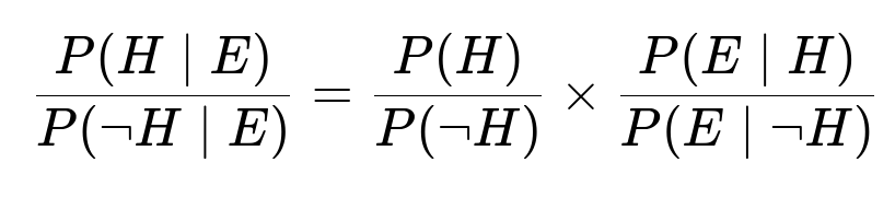
Here:

• P(H) is the prior probability that oil is present (before seeing the test result).

• P(E|H) is the probability that the test is positive given oil is present (true positive rate).

• P(E|¬H) is the probability that the test is positive given oil is not present (false positive rate).

• P(¬H) is 1 – P(H).

• P(H|E) is the posterior probability that oil is present (after seeing the test result).

• The ratio P(E|H)/P(E|¬H) is often called the Bayes factor or likelihood ratio.

Applying Bayes’ Rule Step-by-Step

1. Identify the Prior Probability and Its Complement

   • Prior probability that oil is present: 0.4

   • Therefore, probability that oil is absent: 0.6

   • Prior odds in favor of oil being present: (0.4 / 0.6).

2. True Positive and False Positive Rates

   • Probability of a positive test if oil is present: 0.9 (this is sometimes called “sensitivity”).

   • Probability of a positive test if oil is absent: 0.15 (this is the false positive rate).

3. Compute the Bayes Factor (Likelihood Ratio)

   • Likelihood ratio = (0.9) / (0.15) = 6.

4. Update the Odds

   • Prior odds × Likelihood ratio = (0.4 / 0.6) × 6.

   • (0.4 / 0.6) = 2/3. Multiplying by 6 gives 6 × 2/3 = 4.

   • Hence, the posterior odds are 4 to 1 in favor of oil being present.

5. Convert Posterior Odds to Probability

   • Posterior probability of oil being present = 4 / (1 + 4) = 0.8.

Alternative: Standard Bayes’ Formula

We can also use the more commonly seen version of Bayes’ theorem:

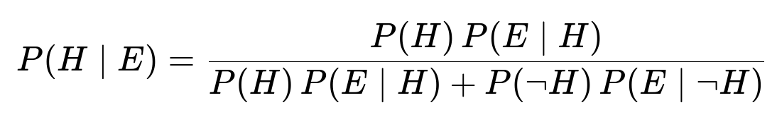
Substituting numerical values:

• Numerator = 0.4 × 0.9 = 0.36

• Denominator = 0.36 + (0.6 × 0.15) = 0.36 + 0.09 = 0.45

• Final probability = 0.36 / 0.45 = 0.8

Both approaches lead to the same answer: 0.8.

Interpretation

After observing a positive test result, the belief that oil is present in the area rises from 0.4 to 0.8. This is because the true positive rate of 90% is quite high compared to the false positive rate of 15%, and the prior probability (40%) was substantial enough to begin with.

Follow-Up Questions

1) Why is the odds form of Bayes’ rule useful?

The odds form shows directly how likelihood ratios scale the prior odds to yield the posterior odds. If you have a test with a certain true positive rate and false positive rate, you can quickly multiply the prior odds by that ratio without having to use the fraction form of Bayes’ rule. In many practical scenarios, odds can be easier to interpret, especially if you have to update multiple pieces of evidence sequentially. Each new piece of evidence corresponds to another likelihood ratio to multiply by, streamlining repeated updates.

2) What are some pitfalls if the prior probability is misestimated?

If the prior probability (here, 0.4) is significantly off from the true underlying probability, then even a highly reliable test can yield a misleading posterior. For example, if the true prior was much lower than 0.4, you might overestimate the chance that oil is actually present after a positive test. Conversely, if the true prior were higher, you might underestimate the reliability of a negative test result. In real-world practice, carefully estimating or updating the prior probability can be crucial, especially when dealing with rare events.

3) How do sensitivity and specificity relate to these calculations?

• Sensitivity refers to P(E|H), the probability that the test is positive given that oil is present. In this example, it is 0.9.

• Specificity is the probability that the test is negative given oil is not present. In this example, specificity is 1 – 0.15 = 0.85.

• These measures determine the likelihood ratio. A high sensitivity (close to 1) and a high specificity (also close to 1) produce a large ratio P(E|H) / P(E|¬H), which strongly shifts the posterior in favor of (or against) the hypothesis.

4) How would you quickly verify this in Python?

Below is a minimal Python snippet showing how one might compute the posterior probability:

prior = 0.4
p_true_positive = 0.9
p_false_positive = 0.15

p_positive_given_oil = p_true_positive
p_positive_given_no_oil = p_false_positive
p_no_oil = 1 - prior

# Using standard Bayes’ formula
posterior = (prior * p_positive_given_oil) / (
    prior * p_positive_given_oil + p_no_oil * p_positive_given_no_oil
)

print(posterior)  # Should print 0.8

This concise code directly implements the standard Bayes’ formula and should yield 0.8 as the final probability.

5) Could we have used frequentist or alternative approaches for this problem?

From a frequentist standpoint, you could treat the test’s 90% and 15% rates as empirical estimates and then calculate the probability of oil using observed data in repeated trials or confidence intervals around these estimates. However, to arrive at a single updated probability that oil is present after observing a positive test, a Bayesian approach is more straightforward and explicitly incorporates your prior belief (in this example, 0.4) into the calculation.

Below are additional follow-up questions

How might the cost of a mistaken decision change the way we use the posterior probability?

A mistake in oil exploration can be expensive. If you decide to drill (acting as if oil is present) but there is no oil, you lose the cost of drilling. Conversely, if you decide not to drill but there actually is oil, you lose the potential profit. In a purely Bayesian calculation, you might only look at the posterior probability of 0.8 and say “it’s likely enough that there is oil.” But in real practice, the financial or strategic implications of being wrong can shift your threshold for deciding to drill.

For instance, suppose it costs tens of millions of dollars to drill but the payoff of finding oil could be hundreds of millions. Even a probability of 0.8 might be compelling. On the other hand, if drilling is extremely expensive and your payoff from striking oil is not as large, you might require a posterior probability much closer to 1.0 before proceeding. This concept is formally captured by Bayesian decision theory, where you incorporate different costs or utilities for each outcome and pick the action that maximizes your expected utility.

What if the seismic test is known to produce inconclusive or borderline results?

In real field operations, a test might yield degrees of confidence rather than a strict positive/negative. For example, there might be “strong positive,” “weak positive,” or “uncertain” signals. If the test result is borderline, you can model it as having different P(E|H) and P(E|¬H) corresponding to each outcome category. For instance, a “weak positive” might have a smaller true positive rate (say 70%) and a smaller false positive rate (say 5%). You could then apply Bayes’ rule to each category of outcome.

A big pitfall arises if people still treat all positives as the same. In practice, a borderline reading might barely differ from background noise. Mislabeling it as a standard positive could inflate your posterior probability erroneously. Thus, you need a more nuanced model that accommodates multiple evidence categories or continuous likelihood functions.

Could repeated tests be performed, and how would that alter the posterior?

Often, companies run multiple seismic tests or use complementary methods (e.g., gravitational or magnetic surveys). If you assume each test is conditionally independent given that oil is present or absent, you can multiply the separate likelihood ratios to get an overall likelihood ratio. Concretely:

• First test: Posterior odds = Prior odds × LR(test1).

• Second test: Posterior odds = (Posterior odds from first test) × LR(test2).

• And so forth.

One pitfall is that these tests might not be strictly independent. If they share common noise sources or the same underlying geophysical data, you could overcount evidence by multiplying likelihood ratios that are not truly independent. This could lead to an overconfident posterior. In practice, experts should estimate or measure the correlation between tests.

How do geographic or geological factors affect our prior probability?

Different geologic basins or formations have vastly different probabilities of containing oil. The 0.4 prior might be specific to one region. If you apply the same reasoning in an area with a historically low discovery rate—perhaps the true probability of oil is only 0.05—then your posterior might still end up too high after a positive test. Conversely, in a highly prolific region where the true prior is 0.8, using 0.4 would lead you to underestimate your posterior probability.

A subtle real-world issue: even within the same region, the geological characteristics can vary from site to site. A single prior probability might not hold across all sites. This is why large exploration firms usually have geologists, geophysicists, and analysts update site-specific priors as more data is gathered about local structures, rock formations, and historical success rates.

How would population-level prevalence of oil affect false positive rates if the test is deployed on many fields?

False positive rate is typically considered a characteristic of the test itself, independent of the prevalence. However, in large-scale deployment, factors such as calibration drift or environmental differences between sites can shift the actual false positive rate away from its nominal 15%. For instance, if certain geological conditions produce signals that mimic oil presence, the effective false positive rate might climb in those regions.

When the test is scaled to many fields, you might observe a pool of “positives” that are heavily influenced by the prior across different locations and the actual test performance in each environment. This phenomenon mirrors the difference between theoretical false positive rate (from controlled test conditions) and real-world performance. Careful recalibration or region-specific test parameters can mitigate this risk.

What if the test accuracy depends on additional factors like well depth or rock density?

A 90% true positive rate might be valid only under certain conditions, such as shallow wells with stable rock properties. In deeper formations or with different lithologies, the test’s performance could degrade. As a result, P(E|H) might be lower than 0.9 or P(E|¬H) might be higher than 0.15.

If the model is not updated to reflect these conditions, the Bayesian update will be misleading. You could address this by having a conditional likelihood: P(E|H, X) and P(E|¬H, X), where X represents factors like depth or density. That way, you tailor the test parameters to local geology. Omitting these factors might lead to an unwarranted belief in test reliability.

Could a negative test still leave a significant chance that oil is present?

Yes. If the test indicates “no oil” (i.e., negative), the posterior probability might still be nontrivial depending on the false negative rate. In the original example, the test’s sensitivity is 90%, meaning there’s a 10% chance of missing real oil. If your prior belief was high—say 0.8—and the test comes back negative, you would do a Bayesian update accounting for that 10% miss probability. The resulting posterior might still be fairly large, perhaps in the 0.4 to 0.5 range, enough to justify further exploratory techniques.

A major pitfall is to dismiss the possibility of oil after a single negative test, especially if the costs of a missed opportunity exceed the cost of further testing.

How might we handle the situation where the test output is not just positive or negative, but a continuous measurement?

Some seismic methods output an amplitude that correlates with the likelihood of oil. Instead of a single probability for “positive,” you have a probability density function for the amplitude under each hypothesis (oil vs. no oil). You can then apply Bayesian updating with a continuous likelihood:

• For any observed amplitude a, compute L1(a) = f(a|H) and L2(a) = f(a|¬H), where f is a probability density function under each hypothesis.

• The posterior odds become prior odds × (L1(a)/L2(a)).

In real-world usage, data might come in as waveforms. You might process them to extract features and produce a posterior distribution for the presence of oil. The subtlety is ensuring that amplitude distributions are well-estimated for various geological conditions. If you incorrectly model these distributions, your posterior estimate can be biased.

Under what conditions would we consider ignoring the test result entirely?

If you have very low confidence in the test’s reliability—e.g., your false positive rate is extremely high, or the test is known to be defective in the current geological setting—you might treat the test result as non-informative. In that scenario, you effectively set P(E|H) = P(E|¬H), making the likelihood ratio equal to 1. Then, your posterior odds remain the same as your prior odds.

This might happen if the test equipment malfunctions or if the data quality is too poor to interpret. A real-world pitfall is that sometimes decision-makers still overreact to a questionable test result due to psychological biases like anchoring on any piece of data.

Is there a scenario where we should update the test performance metrics based on the observed data?

Yes. Bayesian updating can apply not only to the probability of oil but also to the parameters describing test accuracy. If the test is relatively new or tested on fewer sites, you might place priors on P(E|H) and P(E|¬H) themselves, then revise those parameters as you accumulate more real-world test outcomes. This hierarchical Bayesian approach helps you refine both the probability of oil in a given location and the reliability of the test itself.

However, a significant pitfall can arise if you update the test accuracy parameters and the probability of oil simultaneously from a small dataset. This can lead to confounding where the model can’t distinguish whether the test is less accurate or whether oil is just less common. Strong domain knowledge and careful experimental design help reduce such confounding.