ML Interview Q Series: Robust Vehicle Energy Prediction with Failing Sensors Using Huber Loss

📚 Browse the full ML Interview series here.

37. You're working with several sensors designed to predict an energy consumption metric on a vehicle. Several sensors can fail completely. What cost functions might you consider, and which would you decide to minimize in this scenario?

This problem was asked by Tesla.

When dealing with multiple sensors that feed data into a predictive model for a key metric such as energy consumption, you often face significant challenges when some sensors fail outright or produce very noisy or corrupted readings. The issue becomes how to ensure the learning process (training the model) remains robust despite these failures. In typical regression tasks (e.g., predicting a continuous energy metric), common cost functions include Mean Squared Error (MSE), Mean Absolute Error (MAE), Huber Loss, and sometimes custom robust loss functions.

There are specific considerations for why one loss function might be preferred over another when sensors can fail completely or partially:

MSE (Mean Squared Error) is a standard choice for regression but is highly sensitive to outliers. If a sensor produces extreme erroneous values (for example, because it fails and starts returning very large or random readings), MSE heavily penalizes those large errors. This can overly distort parameter updates during training.

MAE (Mean Absolute Error) is more robust than MSE in the face of outliers because it uses absolute deviations instead of squared deviations. However, MAE can be less sensitive in certain regimes, and its gradient behavior can be less stable around zero.

Huber Loss merges the benefits of MSE and MAE. When the errors are small, it behaves like MSE, and when the errors surpass a certain threshold, it behaves more like MAE, reducing sensitivity to outliers.

Robust M-estimators (like the Tukey loss, Cauchy loss, or other specialized robust cost functions) can also limit the influence of large residuals from failing sensors. These cost functions “down-weight” outliers so that a small subset of corrupted sensor readings does not dominate the training objective.

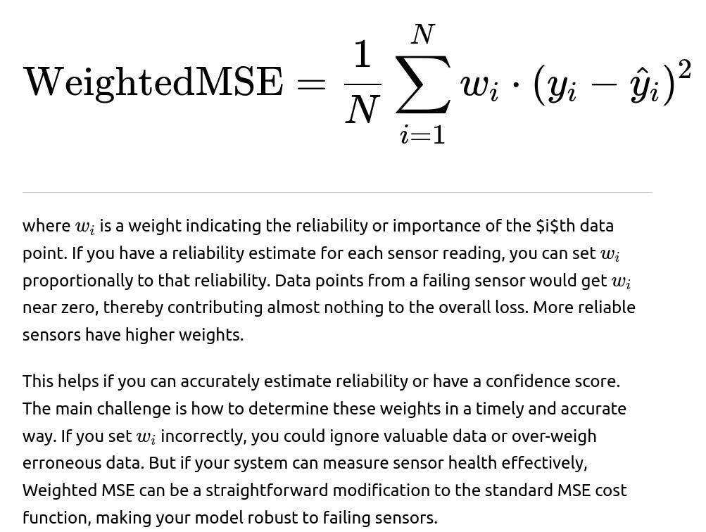
In scenarios with complete sensor failures or partial missing data, you may need a cost function that gracefully ignores or down-weights missing or clearly invalid readings. You might incorporate a per-sensor reliability indicator or gating mechanism, effectively weighting each sensor's contribution. A Weighted MSE or Weighted MAE can be used, but the key is how you assign the weights and handle missingness.

In practice, many organizations end up using Huber Loss or a specialized robust objective that mitigates the effect of extreme outliers caused by sensor failures. Because the question references multiple sensors (some of which may fail completely), the usual recommendation is to minimize a robust loss that can handle extreme outliers in a stable way. Often, this is Huber Loss or a similar function that is easy to implement in most frameworks (PyTorch, TensorFlow, etc.) and provides a good balance between squared error for “normal” readings and absolute error for “outlier” readings.

When deciding precisely which cost function to pick, you consider:

How catastrophic the sensor failures are. If some sensors produce random large readings, MSE alone might be too sensitive.

Whether the computational complexity of certain robust methods is acceptable. Huber is typically not much more complex than MSE or MAE.

Whether you need an explicit weighting scheme that accommodates partial sensor data. You might design a cost function that selectively excludes or weights out failed sensors.

Which performance metric is ultimately used. If your final evaluation uses an R2R2 or MSE-based measure, you might still favor a robust approach for training that leads to better real-world performance.

Overall, many teams in practice would choose to minimize Huber Loss (or a similarly robust variant) because it is a simple, popular, and well-understood compromise between MSE and MAE, and it more gracefully handles large errors due to sensor failure than MSE does alone.

Below is a conceptual representation of Huber Loss:

$$\text{HuberLoss}(r) =

\begin{cases} \frac{1}{2} r^2 & \text{if } |r| \le \delta \ \delta(|r| - \frac{1}{2}\delta) & \text{otherwise} \end{cases}$$

Here, rr is the residual (prediction error), and δδ is a threshold parameter determining the boundary between the quadratic and linear regimes. When the absolute error is small, you get the squared penalty (similar to MSE). When the absolute error is large, the loss becomes linear in the error, reducing outlier sensitivity.

In summary, you might consider MSE, MAE, or specialized robust methods. But given several sensors can fail completely, a robust approach (Huber Loss or a robust M-estimator) is often preferable to reduce the undue influence of sensor failures. Therefore, in many real-world production-grade scenarios, you would likely decide on minimizing Huber Loss.

You can see a simplified example of how you might implement Huber Loss in PyTorch:

import torch
import torch.nn as nn

class HuberLoss(nn.Module):
    def __init__(self, delta=1.0):
        super().__init__()
        self.delta = delta

    def forward(self, predictions, targets):
        errors = predictions - targets
        abs_errors = torch.abs(errors)
        quadratic = 0.5 * errors**2
        linear = self.delta * abs_errors - 0.5 * (self.delta**2)
        return torch.mean(torch.where(abs_errors <= self.delta, quadratic, linear))

# Usage in a training loop
model = ...  # Your model definition
criterion = HuberLoss(delta=1.0)
optimizer = torch.optim.Adam(model.parameters(), lr=1e-3)

for data, targets in dataloader:
    optimizer.zero_grad()
    predictions = model(data)
    loss = criterion(predictions, targets)
    loss.backward()
    optimizer.step()

This example shows how to incorporate a custom Huber Loss class in your training pipeline. If certain sensors are known to fail, you would have an additional step that either masks or imputes invalid sensor data or modifies the cost function to ignore or reduce weight for that data.

A robust cost function can ensure that if a sensor entirely fails and starts producing large outliers, your training will not be dominated by these few large errors, thereby protecting the stability and accuracy of your predictions in real-world deployment.

What if multiple sensors produce contradictory data or large outliers simultaneously?

When multiple sensors are feeding contradictory (and possibly outlier) data, you can still benefit from a robust cost function. However, if a large fraction of sensors fail or produce noise simultaneously, even a robust loss can struggle. You might explore:

Ensuring data sanity checks or pre-processing before feeding to the model. If you can detect the sensor is failing, you can mask or discard those readings at the input level.

Using an architecture that can integrate sensor reliability into the feature representation. For example, you can train a small gating or attention mechanism that learns to weigh sensors that produce consistent data more heavily.

Implementing data-level methods like RANSAC-like procedures, or more advanced robust statistical frameworks, to detect which sensors are outliers in each training iteration.

Evaluating whether some sensor signals are fully redundant, and if so, removing or ignoring them if they appear consistently unreliable.

In each scenario, the cost function is only part of the solution. Robust modeling practices around data ingestion and sensor reliability are also critical.

How would you handle missing data in your cost function when a sensor fails entirely?

In real-world applications, a sensor failure might produce completely missing data. Traditional loss functions like MSE or MAE require numeric predictions and targets. If the target or input is missing for a particular sensor, you need a strategy such as:

Imputation. You can impute the missing value with a learned statistic (mean, median) or through a more sophisticated model that tries to fill in the missing sensor reading from other correlated sensors. The cost function then evaluates how well the imputed reading (and resulting model prediction) matches the ground truth.

Masking in the cost function. A specialized cost function can skip terms associated with missing sensor readings. If you create a partial label scenario, you only compute the loss on sensors or data samples that are valid. The model is then trained with partial observations but can still learn from whichever sensors did not fail.

Using a dedicated approach that explicitly models missingness. Some neural network architectures incorporate an indicator variable “mask” that signals whether a sensor reading is present or not. The model can adaptively adjust its predictions based on which sensors are reliably present.

For each approach, you ensure the cost function does not unfairly penalize missing data, since there is no valid ground-truth reading to compare. Weighted MSE or Weighted MAE can be used, where weights for missing or invalid data are set to zero or a very small value so they do not affect updates.

Could you ever want to keep MSE in this scenario?

One possible compromise is using MSE but applying an outlier rejection or clipping step in the data pipeline. For instance, if sensor readings are known never to exceed a certain physical threshold unless the sensor has failed, any reading beyond that threshold might be clipped or removed. This data-level fix can help MSE remain stable. But this approach can be less elegant and less adaptive than simply using a robust cost function.

How do you tune the δ in Huber Loss?

Tuning δ in Huber Loss is a matter of cross-validation. You pick a few candidate δ values and compare performance on a validation set. The best δδ usually depends on the scale of your typical errors:

A smaller δ makes the loss switch to the linear regime more quickly, so it behaves more like MAE for moderately sized errors. This is more robust but can be slower to converge.

A larger δ means you treat more errors in the quadratic regime, which can give you the benefits of MSE for a wider error range, but can be more sensitive to outliers.

You can start with a heuristic based on the approximate standard deviation of errors or use data-based heuristics. For example, if you expect normal operation to yield errors mostly in the 0 to 2 range, you can set δ=2. Then you iteratively refine it based on performance metrics.

How do you detect that a sensor has failed if its readings seem plausible?

In many real-world sensor systems, you can track a sensor’s operational state or health checks that do not rely solely on data plausibility. This might come from direct health status signals in the sensor firmware, or from comparisons to known redundant sensors.

But if you only have the raw readings, you can implement anomaly detection methods (such as an autoencoder or a moving average filter) to see if that sensor’s outputs deviate sharply from historical or typical operating distributions. If a sensor’s data distribution is drastically different from normal, it might be flagged as failing.

Your cost function alone might not detect a subtle sensor failure if the sensor readings still appear reasonable but are consistently biased. In that case, you might see a noticeable uptick in the training or validation error if that sensor’s input is critical to the model. Monitoring validation metrics for different subsets of sensor usage can also help isolate which sensor might be failing.

How do you ensure your model remains robust if multiple sensors fail at once?

If many sensors fail simultaneously, it can be extremely difficult for the model to maintain accurate predictions. You might consider:

Building redundancy into your sensor suite so that at least some sensors rarely fail at the same time.

Using ensemble methods or multiple models specialized in subsets of sensors. If one group of sensors is present, you use one specialized sub-model; if another group is available, you use another. This approach, however, complicates training and deployment.

Adopting a hierarchical or gating approach that tries to figure out which sensors are still trustworthy, and weighting them accordingly.

In practice, if a large fraction of sensors fail, you may degrade gracefully but still see a performance hit that no cost function alone can fix. Your goal is to design both the data pipeline and the model architecture to handle partial or complete sensor losses in the real world.

Potential pitfalls of using robust cost functions in big data scenarios

While robust cost functions such as Huber or specialized M-estimators help, they can still present challenges in large-scale systems:

They can be more difficult to tune hyperparameters (like δ in Huber or scale parameters in other robust losses).

They might have more complex gradients in certain frameworks, although modern deep learning libraries handle them efficiently in most cases.

They can hide legitimate anomalies if you rely solely on them to filter out outliers. If many readings from a sensor are flagged as “outliers,” you might not see the underlying systematic failure that needs a hardware-level fix.

Despite these pitfalls, robust cost functions remain a very common, practical, and high-impact method in data scenarios involving potential sensor failures.

Example scenario and code snippet

Imagine a scenario where you have 10 sensors measuring different parameters of a vehicle’s operation. You want to predict the energy consumption of the vehicle in the next minute. Some sensors might fail entirely, returning NaN or extremely large values. You preprocess these values either by marking them as missing or clipping them to a safe limit, and then you pass them into your neural network or regression model. You define a robust cost function in your training loop:

import torch
import torch.nn as nn

class SimpleEnergyModel(nn.Module):
    def __init__(self, input_dim, hidden_dim):
        super().__init__()
        self.fc1 = nn.Linear(input_dim, hidden_dim)
        self.relu = nn.ReLU()
        self.fc2 = nn.Linear(hidden_dim, 1)

    def forward(self, x):
        x = self.relu(self.fc1(x))
        x = self.fc2(x)
        return x

# We'll use a built-in HuberLoss (for instance) from PyTorch 1.9+
# If it's not available, we could use the custom version shown earlier.
model = SimpleEnergyModel(input_dim=10, hidden_dim=64)
criterion = nn.HuberLoss(delta=1.0)
optimizer = torch.optim.Adam(model.parameters(), lr=1e-3)

def preprocess_sensor_data(raw_sensors_batch):
    # raw_sensors_batch is a shape [batch_size, 10] tensor
    # Suppose values > 1e6 are considered sensor failures, or nan
    # We'll clip them or set them to zero and keep track of a mask
    # This is just a simplistic example. In practice, you do a more refined approach.
    clipped = torch.where((raw_sensors_batch.abs() > 1e6) | raw_sensors_batch.isnan(),
                          torch.zeros_like(raw_sensors_batch),
                          raw_sensors_batch)
    return clipped

# Training loop
for epoch in range(epochs):
    for batch_sensors, batch_energy in train_dataloader:
        # Preprocess to handle sensor failures
        batch_sensors_prepared = preprocess_sensor_data(batch_sensors)

        predictions = model(batch_sensors_prepared)
        loss = criterion(predictions, batch_energy)

        optimizer.zero_grad()
        loss.backward()
        optimizer.step()

In this simplified example, the model is trained using Huber Loss to reduce the influence of large outliers. The preprocessing step zeroes out (or potentially imputes) any sensor reading that is beyond a certain threshold, treating that reading as effectively “missing.” This approach, coupled with a robust objective function, makes the model more tolerant of sensor failures.

Final choice of cost function in real-world automotive scenarios

Because the question specifically references complete sensor failures, the best practical choice is usually a robust objective that can down-weight or ignore those extreme failure cases. Huber Loss is a common and straightforward solution. Other robust M-estimators or even Weighted MSE with an outlier-clipping pipeline can be viable as well. The key idea is that, given the possibility of large outliers from failing sensors, you minimize a cost function that does not become disproportionately large from those few corrupted samples.

Many teams settle on Huber Loss because:

It is straightforward to implement and interpret.

It smoothly transitions from the squared error region to the absolute error region.

It works well in practice for many tasks.

It remains differentiable everywhere, which is nice for gradient-based optimizers.

Hence, the short, direct answer is that you might consider MSE, MAE, Huber Loss, or more advanced robust cost functions. In a scenario with frequent sensor failures, you would most likely decide to minimize the Huber Loss (or a similar robust function) to handle outliers gracefully.

Follow-up Question: How would you handle a situation where the cost of under-predicting energy consumption (leading to potential system issues) is higher than over-predicting?

When mispredictions carry different costs depending on whether the model underestimates or overestimates the true value, you might design an asymmetric loss function. A typical example is Quantile Loss, where you can place higher penalty on one side of the error distribution. Alternatively, you can modify MSE, MAE, or Huber to have different weights for positive versus negative residuals.

For example, if under-prediction is more costly, you could multiply the part of the loss for negative residuals by a higher factor than for positive residuals. Or you might set a quantile (like 0.8 or 0.9) to ensure you’re systematically aiming for predictions that meet or slightly exceed the actual energy consumption.

You could also adopt specialized cost functions such as a “pinball” loss (used in quantile regression) to heavily penalize underestimates. That helps you produce a model that is more conservative, ensuring it typically errs on the side of over-predicting energy requirements, thereby minimizing the operational risks associated with underestimating.

Follow-up Question: What if the distribution of errors changes over time because the vehicle is operating in different conditions?

If the distribution of errors changes due to seasonal effects, new operational conditions, or sensor aging, even a well-chosen cost function can lead to suboptimal performance. In that case, you would do:

Continuous or online learning, where your model (and cost function) adapt to new data patterns. You might recalculate scaling or weighting factors for the robust loss as distributions shift.

Domain adaptation or transfer learning, so that your model can incorporate new data from changed conditions without forgetting previously learned behaviors.

Periodic retraining using recent data, ensuring that the cost function sees the most up-to-date sensor behavior patterns.

Adaptive thresholding for robust loss parameters. For instance, you might dynamically adjust δ in Huber Loss if the error distributions are drastically shifting.

In practice, sensor drift or changes in environment can be as big a problem as sensor failures. You often combine robust cost functions with a pipeline that regularly evaluates performance and updates the model accordingly.

Follow-up Question: How do you compare model performance across different cost functions in practice?

Comparing performance across cost functions typically involves:

Using a held-out validation or test set of data collected from real (or carefully simulated) operations.

Measuring robustness metrics. Specifically, you can artificially inject sensor failures or outliers in a controlled manner to see how the model’s performance degrades. This helps assess how tolerant the model is under partial sensor failure.

Monitoring real-time performance once the model is deployed. Collect feedback from production usage to see if the robust cost function you chose truly mitigates issues caused by sensor failures.

In an automotive context, the final measure is often whether the system remains safe and stable under partial failure, not just whether the test set MSE is a bit lower. You might track how your predictions differ from the actual energy usage across various extreme conditions (cold weather, steep inclines, or sensor malfunction).

Follow-up Question: Could an ensemble of models each trained with a different cost function be beneficial?

Yes. There is a possibility that an ensemble of models, each trained with a different cost function, can provide a more resilient final prediction. For instance:

One model trains with MSE and learns to capture typical patterns effectively.

Another model uses Huber Loss and remains robust to a certain level of outliers.

Another model uses a heavily outlier-resistant function (e.g., Tukey loss).

Then you combine their predictions (averaging or via a learned meta-learner). Ensembles often improve overall performance, especially if each model captures different aspects of the data distribution and handles sensor failure differently.

However, an ensemble increases the computational burden and complexity in deployment. For real-time systems on vehicles with limited edge computing resources, you might prefer a single robust model. Still, an ensemble is a powerful technique if resources permit.

Follow-up Question: What is a Weighted MSE approach, and why might it help?

A Weighted MSE approach is:

Follow-up Question: How do you implement a custom robust cost function that is not built into common frameworks?

Most deep learning frameworks (PyTorch, TensorFlow) allow you to write custom cost functions by defining a forward pass that computes the loss from predictions and targets. The key is to ensure you:

Use the framework’s tensor operations so you can backpropagate automatically.

Handle potential corner cases: infinite or NaN values, extremely large outliers, or zero denominators.

Return a scalar that you can backward() in PyTorch or minimize() in TensorFlow.

As shown in the example for HuberLoss above, you create a class that extends nn.Module in PyTorch (or a custom function in TensorFlow that uses tf.GradientTape). Inside that class or function, you compute your robust objective element-wise and then average or sum it to get a scalar. The framework then tracks all the operations and computes gradients automatically.

Follow-up Question: How do you scale your robust approach if the data has extremely large ranges of values?

If your data can span multiple orders of magnitude, even robust cost functions can be skewed. Common practice is to normalize or standardize your features and targets (e.g., subtract mean and divide by standard deviation, or use min-max scaling). By scaling your inputs and targets, you bring them into a manageable range where typical error magnitudes are not enormous.

After scaling, your robust loss behaves more predictably. You can also cross-validate the best δ in Huber Loss or other parameters in a standardized range. At inference time, you transform predictions back to the original scale as needed. This approach is standard in many regression problems, especially those dealing with sensor data across wide operating regimes.

Follow-up Question: Could classification-based approaches ever be relevant?

If you bucket your energy consumption metric into categories (low, medium, high consumption), you transform the problem into classification. Then you would use a classification loss like Cross Entropy. This might simplify handling missing or failing sensors in some contexts, especially if you only need to know which consumption range the vehicle is in. However, you lose fine-grained numeric detail about actual consumption.

For critical tasks like precise energy forecasting for range estimation in electric vehicles, classification might be too coarse. You might prefer a direct regression approach or a “soft” classification approach (quantized bins with an ordinal or regression-based perspective). Typically, cost functions like MSE, MAE, or robust variants remain more suitable for numeric predictions unless you have a strong reason to treat the problem in a discrete category manner.

Follow-up Question: Could you use a probabilistic approach, such as a negative log-likelihood?

Yes, you could model the energy consumption as a random variable and use a probabilistic loss function like negative log-likelihood for a Gaussian distribution or some heavy-tailed distribution if you suspect outliers. For instance, you can assume:

Follow-up Question: Is there a difference between sensor-level weighting and sample-level weighting in a Weighted MSE?

Yes. In Weighted MSE, you often see the formula in a sample-level context, where each training example has a single weight that multiplies its entire loss. But in a multi-sensor scenario, each sample might have multiple sensor readings, some of which might fail, while others are valid. If sensor 1 is valid but sensor 2 is not, you might only want to down-weight or ignore the contribution to the loss from sensor 2’s portion of the data, not sensor 1’s. This leads to a more granular weighting approach, perhaps done in the feature space or partial labeling approach.

In some tasks, you have separate partial targets for each sensor. If you only have the “true” energy reading from some subset, you can compute a partial error and average over just the known subset. Weighted MSE can be extended to handle these partial label scenarios by only applying weights to valid sensor-target pairs. That ensures that failing sensors (with missing or invalid data) do not generate spurious gradients.

Follow-up Question: How do you handle the fact that robust losses might slow down learning for normal data points?

Robust losses, by down-weighting large errors, can also be less aggressive at pushing parameters to fix large errors if they are truly legitimate. This can slow convergence. One workaround is to gradually transition from a simpler cost function like MSE to a robust function as training progresses. For example, you can start with MSE for a certain number of epochs, letting the model quickly learn average-case scenarios, then switch to a robust function once the model is somewhat stable, to protect against outliers.

Alternatively, you can carefully tune the parameters (like δδ in Huber or scale parameters in other robust functions) so that normal-range errors are still penalized sufficiently. You can also adopt an adaptive approach that detects how many outliers are present. If the fraction of outliers is small, you can remain fairly strict; if it’s large, you can become more robust.

Follow-up Question: How does your choice of cost function interact with the optimizer?

The choice of cost function interacts with the optimizer primarily through the gradient shape. MSE yields gradients that grow with the error magnitude. MAE yields a constant gradient magnitude (for non-zero errors), which can lead to slow or unstable training near zero residual. Huber Loss yields gradients that are linear for large errors but scale with the residual for small errors, giving a compromise behavior.

Most optimizers (SGD, Adam, RMSProp) can handle these losses without any problem. However, if your cost function has non-smooth points (like the absolute value in MAE), that can lead to subgradient approaches in those exact points. Modern frameworks handle this gracefully, but it can still affect convergence speed or stability. In practice, Huber or a smooth robust cost is often easier to optimize than pure MAE. Meanwhile, MSE remains the simplest in terms of gradient shape, but again is less robust to outliers.

If you find training is unstable, you might reduce the learning rate or experiment with a different optimizer or learning-rate schedule. This is particularly important with custom robust losses that might have more complex gradients than standard MSE.

Follow-up Question: Could you combine advanced neural architectures with your robust cost function to further mitigate sensor failures?

Yes. You can build architectures that explicitly handle missing or failed sensors. Examples include:

Attention-based models that learn to place higher weights on sensors with consistent readings and lower weights on failing sensors.

Mixture-of-experts architectures, where each expert is specialized to handle a certain subset of sensors, and a gating network decides which expert to trust at inference time.

Graph neural networks where each sensor is a node, and you learn to propagate relevant information from reliable sensors to the final prediction. If a sensor is failing, the graph structure can reduce its influence on the overall output.

These architectural choices, combined with a robust cost function (like Huber Loss), can provide a comprehensive solution for sensor-failure scenarios. The cost function ensures outliers do not dominate training. The architecture ensures the model can route around failing or missing sensors dynamically.

Follow-up Question: Are there any real-world results showing the effectiveness of robust cost functions in automotive settings?

Numerous case studies in self-driving car companies, EV battery management systems, and advanced driver-assistance systems (ADAS) have documented scenarios where robust cost functions improved reliability. While exact data might be proprietary, the general consensus is that robust approaches reduce sensitivity to spurious or extreme inputs, leading to more stable performance under partial sensor failure or environmental extremes. In some public academic research, results show that Huber or other robust losses can maintain better predictive accuracy in the presence of artificially injected sensor noise or outliers.

Ultimately, your model’s success depends on:

Quality of data preprocessing and sensor health checks.

Choice of cost function that aligns with your real-world error distribution and risk tolerance.

Appropriate architecture and training procedures that can adapt to incomplete or faulty sensor inputs.

All of these must work together to deliver a system that is not easily derailed by sensor failures.

---

Below are additional follow-up questions

How do you handle random intermittent sensor failures that happen over time, rather than permanent failures?

When sensor failures are intermittent, the sensor might alternate between providing valid measurements and invalid or noisy readings. This introduces a temporal dimension to the problem. A robust cost function helps, but you also need a strategy that accounts for time dependencies:

You can integrate a recurrent or time-series model, such as an LSTM or GRU, to detect patterns in the sensor’s reliability. If a sensor starts producing abnormal readings for consecutive time steps, the model can learn to discount that sensor’s contribution during those intervals.

You can apply an online anomaly detection method on each sensor to trigger a “fail state” whenever a sensor’s readings deviate too strongly from its historical norm. This flag can act as a mask that either removes or down-weights the sensor’s contribution in the cost function.

A potential pitfall is over-reliance on short-term anomalies. If a sensor exhibits short spikes that are not actually failures but legitimate unusual readings, you risk discarding valuable data. One solution is to use a tolerance window that waits for consistent anomalies across several time steps before marking a sensor as failed.

Another subtlety is deciding how quickly to trust a sensor again once it recovers. Some systems impose a “cool-down” period during which the sensor’s readings are gradually phased back into the model. This prevents flip-flopping between “failed” and “active” states if the sensor is unstable.

In practice, a combination of time-series models, anomaly detection, and robust loss functions can help handle random intermittent failures. You log sensor state transitions and continuously monitor the model’s performance to ensure the strategy remains effective.

Could a multi-task learning approach be used to detect sensor failures and predict energy consumption simultaneously?

You can combine sensor-failure detection as one task and energy consumption prediction as another. A multi-task architecture can learn shared representations that help it judge whether a sensor is malfunctioning. For instance:

A shared backbone network takes all sensor inputs. Two heads branch out: one head predicts the vehicle’s energy consumption, and another head outputs a binary or multi-class label indicating whether each sensor is healthy, partially failing, or failed.

The cost function is then a sum (or weighted combination) of a robust regression loss (e.g., Huber) for energy consumption and a classification loss (e.g., Cross Entropy) for the sensor health detection. If you suspect sensor health classification might share underlying feature representations with energy consumption, this approach can lead to better performance on both tasks.

A potential edge case is that if you do not have reliable labels indicating sensor health, the multi-task approach can struggle. In that scenario, you might rely on heuristic or unsupervised methods to generate pseudo-labels for sensor reliability, which may or may not be accurate.

Another subtlety is ensuring that your network does not learn to dismiss a partially failing sensor entirely if it still provides valuable data some fraction of the time. Balancing the weighting of tasks in the multi-task loss is crucial. Too much emphasis on sensor failure detection could overshadow the main regression objective, or vice versa.

How do you decide whether to exclude a failing sensor entirely or try to salvage its data via robust methods?

In some cases, a sensor might degrade to the point where it produces mostly random or implausible values. If the sensor’s data consistently harms the model’s performance, you might opt to exclude it altogether. This decision involves several considerations:

Engineering or domain knowledge. If the sensor’s mechanical or electrical failure mode is known to produce purely random values, you might gain nothing by including it.

Statistical thresholding. If the sensor’s correlation with the target (energy consumption) or its correlation with other sensors’ signals drops below a certain threshold, you might remove it from the model inputs.

Impact analysis. You can perform an ablation study to see how the model’s validation error changes if you exclude that sensor. If performance remains the same or improves, removing the sensor might be beneficial.

A potential pitfall is prematurely excluding a sensor that fails sporadically. If the sensor recovers or if only part of its readings are invalid, you lose potentially valuable information by completely discarding it. A robust cost function that down-weights extreme outliers might be sufficient to handle partial failures without excluding the sensor entirely.

Edge cases arise when you have limited redundancy—if that sensor is your only measure of a critical variable, it may be risky to discard it. You might then attempt advanced imputation techniques, or partial weighting, or keep the sensor’s data in a specialized fallback mode.

What hardware-level or system-wide approaches can you combine with robust cost functions to mitigate sensor failures?

While robust cost functions in machine learning help handle corrupted data, hardware or system-level strategies can further reduce the impact of sensor failures:

Redundancy in sensor design. Having multiple sensors that measure the same or correlated physical quantities ensures at least one sensor typically remains reliable. The model can learn to rely on the redundant sensor data if one fails.

Error-correction or data validation at the sensor firmware level. Some sensors can perform self-checks, calibration, or generate health status codes. The model then has explicit signals indicating sensor health, making it easier to discard or down-weight data from failing sensors.

Regular sensor maintenance schedules. Physical sensors can degrade over time. Routine calibration can minimize large drifts that the robust cost function would otherwise have to handle.

A real-world pitfall is assuming that hardware redundancy alone solves the software problem. Even with multiple sensors, if they share the same vulnerability or are placed in the same environment, a single event can cause multiple failures. This is why software-level robust methods remain important.

An edge case is that sometimes hardware solutions introduce biases if, for example, multiple sensors share the same communication bus that fails intermittently. You might see correlated failures, which requires your cost function to handle wide-scale data corruption at once.

How do you handle gradual sensor drift or aging rather than sudden failures?

Sensors often degrade gradually. Readings may remain within a “plausible” range but systematically shift away from the true value. Such drift is more insidious than abrupt failure because it is harder to detect:

One way is to maintain a rolling baseline or reference for each sensor. If the sensor’s average reading for a known stable operating condition changes over time, you detect drift. Once drift is identified, you can recalibrate or apply a correction factor.

You can incorporate a model that estimates each sensor’s bias or drift. This becomes an additional parameter in training. A robust cost function can help detect that certain sensors have systematically higher or lower residuals, which might indicate a drift.

The main pitfall is letting the model adapt too freely to drift that is actually an indicator of a real phenomenon. For example, if the vehicle’s normal operating temperature environment changes because it’s being deployed in a new climate, the sensor reading shift may be legitimate, not a hardware drift.

Another subtlety is deciding how quickly to adjust the model’s parameters to compensate for drift. If you overreact, you might chase noisy variations. If you underreact, you accumulate large systematic error. This tradeoff often calls for well-designed online or continuous training approaches, combined with robust detection of abnormal sensor shifts.

What if repeated sensor “failures” actually reflect new, valid operating conditions rather than true failures?

Sometimes, what appears to be an outlier might be the system entering a novel state. For example, if the vehicle is operated under extreme environmental conditions for the first time, the sensor readings might fall outside the previously observed range but still be correct. In such cases:

A robust cost function can incorrectly view these new values as outliers and down-weight them. That could slow the model’s ability to learn from newly introduced operating regimes.

You can employ an online learning scheme that attempts to detect if an outlier is truly spurious or if it represents a genuine shift in data distribution. Techniques like a concept drift detector can differentiate between random noise and a systematic, persistent change.

A pitfall is systematically ignoring valid extremes that the model needs to adapt to. If your domain knowledge suggests that certain high or low sensor readings are physically possible (though rare), you need a plan for incorporating them rather than discarding them as failures.

This edge case highlights the tension between robust cost functions (which protect against spurious outliers) and the need to learn from novel, extreme but valid data. A balanced approach might be to track how frequently or consistently “outlier” readings occur. If these readings persist, the model updates its understanding that these values belong to a new normal regime.

How might domain knowledge about vehicle physics help design a more effective cost function for sensor failures?

Domain knowledge can inform constraints or relationships among sensors. For instance, if you know that sensor A and sensor B measure correlated quantities (like engine temperature and coolant temperature), then a drastic mismatch might indicate that one of them has failed:

You can build a physics-inspired model that enforces these relationships or punishes violations of known constraints in the cost function. For example, you add a penalty term if sensor readings violate a thermodynamic limit or a known operational boundary.

A potential pitfall is that real systems can occasionally operate outside idealized domain constraints. Overly strict constraints might label legitimate but rare events as invalid, preventing the model from learning about critical edge cases.

Another subtlety is that domain rules might be approximate. For example, aerodynamic drag depends on speed, air density, vehicle shape, etc. If you embed a simplified formula in the model, you risk ignoring real-world complexities. A partial compromise is to use domain knowledge to guide the choice of robust function thresholds or to define gating logic for sensor reliability.

Could a Bayesian approach that encodes sensor-failure priors yield better robustness than classic cost functions?

A Bayesian model can incorporate prior beliefs about the probability of sensor failure or the expected distribution of outliers. This approach can adapt as it accumulates evidence that a sensor is malfunctioning:

You can define a hierarchical model where each sensor’s readings are drawn from a distribution whose parameters are influenced by a “fail vs. healthy” latent variable. If the model infers a sensor is failing, it updates that sensor’s contribution to the likelihood accordingly.

The cost function becomes the negative log-likelihood of the entire Bayesian model, factoring in sensor failure probabilities and robust data likelihood terms (e.g., heavy-tailed distributions). This approach can automatically “down-weight” data from sensors inferred to be in a failing state.

A potential challenge is the computational overhead of Bayesian inference. Sampling-based methods (like MCMC) or approximate variational methods can be expensive, especially if you have a large number of sensors and high-dimensional data.

An edge case is that if your prior assumptions are incorrect, the Bayesian model might systematically misidentify failing sensors or fail to adapt to unusual but valid sensor readings. Calibrating the prior distribution to match real-world sensor behaviors is critical. If you overestimate failure probability, you might discount valid data too often.

How do you deal with partial ground-truth data for energy consumption or inconsistent labeling across sensors?

In real deployments, you may not always have a perfect energy consumption label for every training example. Sometimes the logging system fails, or you only measure the target variable under certain conditions:

You might use semi-supervised or weakly supervised approaches, training the model with labeled data where available, and using unsupervised consistency losses for unlabeled samples.

If some subsets of data have partial sensor readings and partial labels, you can adopt a multi-head model, training one head on fully labeled data and another on partially labeled data, aligning their features. A robust cost function still helps with outliers, but you also have to handle missing labels.

A risk is that you overfit to the small subset of fully labeled data, ignoring the distribution shift in unlabeled or partially labeled data. Regularization and careful weighting of the different training losses can mitigate this.

Another subtlety is that partial labeling might correlate with sensor failures: if a sensor fails, you might not have a corresponding energy reading. This can bias your training set distribution. You need to ensure your model doesn’t implicitly learn spurious correlations between “missing target label” and sensor states.

What happens if you must predict energy consumption in real-time on limited hardware, and robust cost functions are more complex?

Real-time inference on embedded platforms (like in a vehicle) often requires efficient models. Though robust cost functions typically have comparable computational cost to MSE or MAE, certain advanced robust methods (like complex M-estimators or Bayesian approaches) can be more expensive:

You must ensure your chosen robust loss function doesn’t introduce significant latency. Huber Loss is still relatively cheap, but heavily iterative or sampling-based methods might be too slow.

An alternative is to keep the robust training approach in the cloud or offline environment, then deploy a simpler model for real-time inference. This means the complexity primarily stays in training, and inference remains fast. As new data comes in, you periodically retrain offline with a robust approach, then update the deployed model.

One pitfall is that if your cost function is drastically simplified for real-time usage, you might lose the benefits of robust training. Another edge case is that if sensor failure must be detected and mitigated in real-time, you need at least a lightweight gating or anomaly detection method that can run on the embedded device.

Balancing these constraints is important in automotive contexts where computational resources can be limited, and reliability and low latency are paramount.

How do you validate that your robust sensor-failure handling actually works under real production conditions?

Validation goes beyond standard hold-out test sets. You create test scenarios that mimic real sensor failures or degrade sensors artificially to see how your system behaves. For instance, you can do:

Hardware-in-the-loop (HIL) testing. You inject noise or override sensor signals in a controlled environment to replicate failures and measure how well the model maintains accurate predictions.

Field trials. You deploy in a test fleet or environment with known patterns of sensor failures to gather data on real operational performance.

Synthetic data augmentation. You add artificial outlier patterns or random dropouts to the training data to simulate failing sensors. Then you evaluate if the robust cost function can maintain stable predictions under these conditions.

A subtlety is ensuring you do not rely solely on synthetic failures, because real sensor failure modes can be more unpredictable. You should also measure how quickly the model recovers if the sensor starts returning normal data after a failure.

A potential pitfall is that the model might appear robust in short tests but fail during lengthy operations with complex failure modes. Continuous monitoring of production logs is crucial. You track both short-term (immediate reaction to failure) and long-term (system stability over hours or days) behaviors.