
ML Interview Q Series: ROC Curve Invariance: Effect of Monotonic Transformations Like Square Root on Scores.

📚 Browse the full ML Interview series here.
Assume we have a classifier that produces a score between 0 and 1 for the probability of a particular loan application being a fraud. Say that for each application’s score, we take the square root of that score. How would the ROC curve change? If it doesn’t change, what kinds of functions would change the curve?
This problem was asked by Affirm.
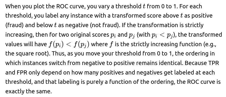
When dealing with ROC (Receiver Operating Characteristic) curves, one of the most fundamental points is that the ROC curve depends solely on the relative ordering (ranking) of the predicted scores for the positive and negative classes. Given any set of predicted scores (for instance, probabilities of being “fraudulent” vs. “not fraudulent”), the ROC curve is created by sweeping a threshold across all possible score values and computing the True Positive Rate (TPR) and False Positive Rate (FPR) for each threshold. Formally:
TPR (also known as sensitivity or recall) measures the proportion of actual positives that are correctly identified as positives.
FPR measures the proportion of actual negatives that are incorrectly identified as positives.
The crucial insight is that the ROC curve is invariant under any strictly monotonic transformation of the scores.
A monotonic transformation is simply a function that changes your scores while keeping their order the same. This means if you have two scores and one is higher than the other, it will still be higher after the transformation.
For example:
If you multiply all scores by 2 (e.g., turning 2, 3, 5 into 4, 6, 10), the order remains the same.
Similarly, if you take the logarithm of all scores (assuming they're all positive), the relative order of the scores doesn't change.
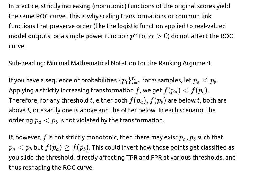
The statement "The ROC curve is invariant under any strictly monotonic transformation of the scores" means that because the ROC curve is based on how well the scores rank the instances (from most likely positive to most likely negative), changing the scores with any function that preserves their order will not alter the ROC curve.

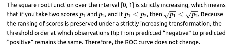
So if we apply the square root to each probability p∈[0,1], we do not alter the ordering of the scores. As a result, the ROC curve stays exactly the same.
This leads to a more general statement: the only kinds of transformations that would change the ROC curve are those that change the relative ordering of the scores. For instance:
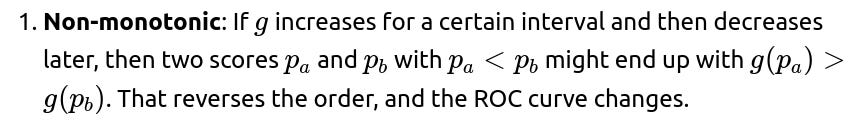
A function that is not strictly monotonic (e.g., a function that increases in one region, then decreases in another).
A function that “flattens” or “lumps together” distinct values into the exact same score for different inputs (e.g., a step function that assigns the same output for a range of different input values, thereby changing relative orderings among scores).
A function that swaps the ordering of two or more data points in some region (e.g., a function that is decreasing over certain intervals in [0,1]).
Below are some extended discussions and potential follow-up questions that might arise in a rigorous interview setting.
Sub-heading: Why the Square Root Transformation Does Not Change the ROC Curve
Sub-heading: What Kind of Functions Would Affect the ROC Curve?
Any function that breaks the strict ordering of scores can affect the ROC curve. For instance, suppose you have a function g(⋅) that is:

Many-to-one (with no internal ordering): If you transform a range of input scores into a single constant output, then you lose granularity among those scores. This changes how thresholds split positives and negatives because distinct points in the original space might become indistinguishable in the transformed space, thus altering the ROC curve.
Not defined on the entire interval or includes discontinuities: For example, a piecewise definition that flips the relative order within certain subranges.

Sub-heading: Effects on Calibration vs. Ranking

Sub-heading: Example Implementation in Python (Measuring ROC)
Below is a code snippet to illustrate how one might measure and plot an ROC curve in Python using scikit-learn. Note how we can plot two curves (one using the original scores, one using a strictly monotonic transformation) and show they match.
import numpy as np
import matplotlib.pyplot as plt
from sklearn.metrics import roc_curve, auc

# Example: We generate random probabilities and simulate ground-truth labels
np.random.seed(42)
y_true = np.random.randint(0, 2, size=1000)         # Ground-truth labels
scores_original = np.random.rand(1000)              # Original scores in [0, 1]
scores_sqrt = np.sqrt(scores_original)              # Transformed scores

# Compute ROC for original
fpr_orig, tpr_orig, _ = roc_curve(y_true, scores_original)
roc_auc_orig = auc(fpr_orig, tpr_orig)

# Compute ROC for sqrt-transformed
fpr_sqrt, tpr_sqrt, _ = roc_curve(y_true, scores_sqrt)
roc_auc_sqrt = auc(fpr_sqrt, tpr_sqrt)

plt.figure()
plt.plot(fpr_orig, tpr_orig, label=f'Original ROC, AUC={roc_auc_orig:.2f}')
plt.plot(fpr_sqrt, tpr_sqrt, label=f'Sqrt ROC, AUC={roc_auc_sqrt:.2f}', linestyle='--')
plt.plot([0,1], [0,1], 'k--')  # diagonal line
plt.legend()
plt.title('ROC Curves: Original vs. Sqrt Scores')
plt.xlabel('False Positive Rate')
plt.ylabel('True Positive Rate')
plt.show()
In this code snippet, the AUC and the shape of the ROC curve (i.e., the relationship between FPR and TPR) remain essentially identical when using the original scores vs. the square-root-transformed scores. The reason is that the relative order of the samples is the same.
Sub-heading: Potential Pitfalls and Edge Cases

Extreme Binning: If someone used a binning function that lumps many different pp values into a single bin, you lose the resolution among those points. This changes the rank order among points that got lumped into the same bin, which might in turn alter the ROC curve because multiple data points would end up having exactly identical scores.
Usage in Production: In a real system that detects fraud, applying transformations to your predicted probabilities might confuse or mislead stakeholders who interpret these as direct probabilities. If a risk management team or compliance team expects a calibrated probability of fraud, a transformation like a square root is inappropriate unless you also re-calibrate your outputs. But from a purely classification-threshold perspective, the ROC remains the same with a strictly monotonic transformation.


Below are several possible follow-up questions and their detailed answers that an interviewer might ask to ensure you truly understand the underlying concepts.
If the ROC curve is not affected by the square root transformation, would something like taking the absolute value of (score - 0.5) affect it?
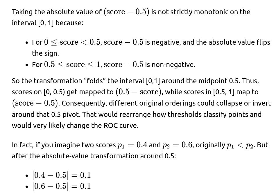
They become exactly the same transformed score, losing the ordering altogether. Meanwhile, points below 0.5 and above 0.5 can get mapped into the same or reversed intervals of the transformed space. Hence, the ROC curve would change.
Does a strictly monotonic decreasing function preserve the ROC curve?
Therefore, in principle, a strictly monotonic decreasing transformation preserves the geometry of the ROC points except it might flip how you normally set thresholds (you would threshold from the top instead of from the bottom). If you are careful and sweep the threshold in the direction consistent with the transformation, you can obtain the same ROC curve shape. The ordering is reversed, but the shape and area remain unchanged.
In practice, how does this relate to the Area Under the ROC Curve (AUC)?
The Area Under the ROC Curve (AUC) is a ranking-based statistic. By definition, it measures the probability that a randomly chosen positive instance is assigned a higher score than a randomly chosen negative instance. Therefore:
Any strictly monotonic transformation preserves which positive vs. negative pairs have higher scores, so the AUC remains the same.
If a transformation changes that ordering even for a small set of pairs, you might see changes in the AUC.
One subtlety arises if your function maps a large set of distinct scores to exactly the same value (like a step function). You might see an increase in the number of tied scores between positives and negatives, which can alter how the AUC is computed for ties. As a result, the AUC might change in that scenario.
Why do some interviewers focus on transformations of model outputs and their effect on ROC curves?
Interviewers often use questions like this to probe your understanding of ranking-based metrics and calibrations. By walking through the mental reasoning of whether a transformation is strictly monotonic, you demonstrate an understanding of:
How threshold-based classification metrics (TPR, FPR) are computed.
The difference between rank-based measures (like ROC) and probability calibration measures (like Brier score or calibration curves).
The potential pitfalls of transforming scores in real-world settings where interpretability or calibration might matter more than pure ranking.
They might also be probing your familiarity with advanced production use cases. For example, in certain explainability or compliance contexts, you cannot simply warp your model’s probability outputs arbitrarily without re-checking the calibration. Even if the ROC curve is not affected, other aspects of the system might be.
Could you provide an example of when preserving the ROC curve but changing probabilities drastically might be problematic?
Consider a financial institution that uses a model’s probability output to determine the interest rate or required collateral for a loan. Even though the model might have an excellent ROC curve, if you apply a transformation such as taking the square of the probabilities or the square root of the probabilities, you change the numerical values.
Suppose the model originally says an application has a 0.30 probability of fraud (meaning a 30% chance). That might be borderline but still considered possible for manual review.
After taking the square root, the score becomes approximately 0.5477, which is much higher than 0.30. If your internal policy says, “Above 0.50, we flag it immediately,” that transformation might escalate a lot more loans to a flagged status—contrary to how the original calibrated scores were intended to be used.
This sort of mismatch would cause confusion in production, especially if risk officers are under the impression that your system outputs “true probabilities” of fraud. The ranking portion (driving the ROC) might be fine, but you lose the well-calibrated interpretation of the probabilities. This can have significant business and ethical consequences.
Is there a scenario where a monotonic transformation might slightly affect the ROC curve due to finite numerical precision?
In theory, a purely mathematical strictly monotonic function cannot change the ROC curve. However, in practical computation with floating-point arithmetic:
Very small differences between scores might become identical after transformation if they were close enough in the floating-point representation. For example, if two distinct probabilities 0.9000000002 and 0.8999999998 become exactly the same value after a transformation, you might inadvertently merge what used to be two distinct ranks into a single rank.
These effects are generally extremely small, but for a large dataset, you could see a tiny difference in how thresholds are enumerated in the ROC computation.
In most real-world applications, such floating-point issues do not noticeably alter the ROC curve. The changes, if any, are typically negligible.
Summary of Core Reasoning
The ROC curve remains invariant to strictly monotonic transformations of the model score because the ranking of the scores for positive vs. negative instances does not change. The square root function in [0,1] is strictly increasing, so it does not alter the rank ordering of scores, leaving the ROC curve intact.
However, non-monotonic transformations or transformations that merge previously distinct values into a single value can reorder or merge data points in a way that changes the ROC curve. Practitioners must also remember that even if the ROC curve remains unaffected, the interpretation and calibration of the transformed probabilities can be drastically different, so transformations must be applied with care in production settings.
Additional Follow-up Question: Are there any differences when analyzing the Precision-Recall curve instead of the ROC curve?

The PR curve also depends on the ordering of scores among positive and negative instances. For the same reason as with the ROC curve, a strictly monotonic transformation of the probabilities should not affect the shape of the Precision-Recall curve or its Area Under the Curve (AUPRC).
However, the PR curve can sometimes reveal different performance aspects compared to the ROC curve, especially in heavily imbalanced datasets (like fraud detection). The ROC curve can look artificially optimistic if there are many negatives. The PR curve is more sensitive to changes in how many false positives you get among a small set of true positives, so many real-world fraud detection tasks rely on PR curves and precision@k metrics more heavily.
Despite these differences in usage, the property that strictly monotonic transformations preserve rank ordering (and thus preserve how thresholds split the data) still applies to the PR curve.

Thus, the essential conclusion is the same for PR curves vs. ROC curves, but the context in which each curve is used may differ significantly in real fraud detection or other highly imbalanced scenarios.
Below are additional follow-up questions
If we use a piecewise linear transformation that is strictly increasing overall but has different slopes in different intervals, will the ROC curve remain unchanged?
A piecewise linear transformation that remains strictly increasing across the entire [0, 1] interval will not change the ROC curve. The essential determinant is that the relative ordering of scores remains intact. Even if the slope in different subranges varies, as long as for any pair of original scores (p_i < p_j), the transformed values still satisfy (f(p_i) < f(p_j)), the thresholding sequence does not change.
However, one subtlety lies in any “kinks” or corner points in your piecewise function. If these “kinks” do not cause a reversal of order, you will still preserve the rank order. Therefore, the ROC curve remains the same. But you need to ensure there are no intervals within which the function is not increasing or is constant. Any portion that is flat would collapse multiple original scores to a single value, which could then merge or reorder them in the sorted list used to compute TPR and FPR. For instance, if in one subrange the function is a constant (slope = 0), then all original scores that fall into that region get mapped to the same number, losing any distinction among them. This loss of granularity might change the ROC curve.
The main takeaway is that strict monotonicity from 0 to 1 (without reversal or constant segments) preserves the ROC curve. A piecewise linear function that is strictly increasing everywhere meets this criterion.
How would adding random Gaussian noise to the scores before thresholding affect the ROC curve, and why might this be done in practice?
When you add random noise to predicted scores, you often disrupt the original ordering unless the noise has a zero-mean and a negligible standard deviation compared to the scale of the differences among scores. In practice, even small noise can reorder some pairs of data points, especially those whose original predicted scores were very close. This means the ROC curve might change slightly, especially around threshold regions where many data points bunch up in the same range.
Why might an organization add noise deliberately? One reason is to break ties. In large datasets, many observations might receive exactly the same model output. This can make threshold selection or certain ranking-based computations cumbersome if you must handle many ties. Introducing a small amount of noise breaks those ties consistently. In such a scenario, if the noise is small enough that it rarely flips the order of points that were clearly separated, the resulting ROC curve usually remains very close to what it was, though technically it can shift slightly.
Another reason is differential privacy or anonymity. In some regulated industries, institutions might add controlled noise to the outputs to mask exact predictions. This can help preserve privacy in model outputs. However, the organization must accept the possible small changes in TPR and FPR due to reordering of close scores.
What happens to the ROC curve if the transformation is monotonic in one region of [0,1] but constant or decreasing in another part?
Any constant or strictly decreasing portion of the transformation will affect the rank ordering. Let’s break down two scenarios:
Transformation is constant over some subrange: All scores in that subrange map to the same output. Distinct original scores within that subrange become indistinguishable. If some of them were positive examples and others were negative, the threshold-based splits in that region might change. You lose the ability to rank-order them. The ROC curve can shift because the transitions between TPR and FPR that used to occur at different scores can merge into a single jump.
Transformation is strictly decreasing in some subrange: If in any portion you invert the order of the scores, you might end up classifying what used to be a higher-valued instance (originally thought more likely to be fraud) below a lower-valued instance. This can lead to substantial changes in the pairs of positive vs. negative scores that get labeled positive at each threshold. As a direct result, you alter the shape of the ROC curve.
Therefore, once strict monotonicity is broken in any segment, the ROC curve can be impacted in that segment and overall.
Could a strictly monotonic transformation be constructed such that it is monotonic but extremely steep in some sections, effectively creating a near-binary output, and what would happen to the ROC curve?
Yes, it is possible to construct a function that is nearly flat in some regions and nearly vertical in others while still being globally increasing. If it never strictly inverts or plateaus completely, you will maintain the rank ordering. In principle, the ROC curve remains the same.
However, in practical numerical terms, a steep region might map many close original scores to widely separated values, and a nearly flat region might map many different scores to very similar values. For example:
In a steep region, slight differences in original scores could become large differences in transformed scores, making that area numerically sensitive to small floating-point deviations or model jitters.
In a flat region (though not strictly constant), distinct scores might bunch together in the transformed space.
As long as the function is strictly increasing, the overall ordering does not change. But from a computational perspective, heavy compression or dilation of certain intervals might introduce numerical artifacts or cause partial ordering issues if floating-point round-off lumps scores together. Technically the theoretical ROC curve is unchanged, but in real implementations, the extremely steep segments might cause difficulty in stable threshold computations.
In a real fraud detection setting, why might we still care about a transformation that doesn't change the ROC curve?
Even if a transformation does not affect the ROC curve, it can still matter a great deal in practice because:
Calibration: Stakeholders often want a probability that truly represents a real-world likelihood. For instance, if a loan has a “20% chance” of being fraudulent, teams may need that to be statistically meaningful, not just a rank-ordering. A square-root or exponential transform can break that calibration.
Risk-Based Thresholds: Banks or lending institutions might set threshold rules, such as “Flag if the probability of fraud is above 0.3.” If you apply a transformation that changes that numeric scale, the same threshold might no longer reflect a “30% chance” of fraud. This can unintentionally alter policies.
Interpretability: Lenders or compliance officers may expect outputs to be interpretable probabilities. A heavily distorted mapping from model output to displayed score might cause confusion or mistrust among users.
Downstream Models: Sometimes the output of one model is fed into another system or used in logistic or linear models for further risk aggregation. A monotonic transformation could disrupt how other components interpret the numeric range, even if the rank ordering remains the same for the immediate classification step.
Thus, from a purely classification metric standpoint, your ROC curve is safe under monotonic transformations. From a production and business standpoint, transformations can have significant consequences, which is why one must be careful applying them.
Could transforming scores change other metrics like the F1 score or accuracy at a fixed threshold?
Yes. While the ROC curve itself is threshold-agnostic (it considers all possible thresholds), many other metrics rely on a specific, pre-chosen threshold. For example:
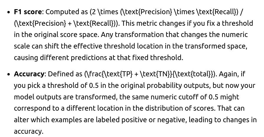
Hence, while the ranking-based metrics (ROC, AUC) remain invariant, any fixed-threshold measure can be heavily affected by the transformation.
If a transformation is monotonic but squashes all scores into a narrow range (like 0.49 to 0.51), how might that impact practical thresholding and real-world usage?
Although such a transformation does not alter the ROC curve in principle, it poses practical difficulties:
Threshold Sensitivity: If almost all transformed scores lie in a tight range, small threshold changes can cause large swings in TPR and FPR. For example, if 90% of your samples are mapped to roughly 0.50, then a threshold of 0.495 might label almost everything as positive, whereas a threshold of 0.505 might label almost everything as negative.
Limited Interpretability: Seeing nearly all scores around 0.5 can confuse business stakeholders. They may interpret the model as being extremely uncertain. In reality, the model might be more confident on certain examples, but the transformation hides that confidence.
Implementation Complexities: Trying to set stable thresholds in production becomes tricky. Even minor floating-point drift might change a large fraction of classifications if the distribution is extremely dense around a narrow band.
Thus, while the theoretical ROC curve is unchanged, the transformation can make it nearly impossible to use threshold-based decisions in a stable manner. Many real-world systems require a more interpretable and spread-out distribution of scores to function smoothly.
Would a monotonic transformation that flips the meaning of scores (like mapping higher scores to lower values but still preserving order among positives and negatives) keep the ROC curve if we interpret it differently?
A transformation that is strictly decreasing overall will reverse the raw order of the scores. If your thresholding convention remains “above threshold = classify as positive,” then your classification logic flips. That would produce a mirrored form of the ROC curve if you keep applying the threshold from 0 to 1 in the usual direction. However, you can recover the same TPR-FPR pairs by reversing how you sweep the threshold (essentially going from 1 down to 0 instead of 0 up to 1).
Hence, if you handle the threshold search properly, you can construct the same set of TPR-FPR points, and the ROC curve shape is identical. In a practical sense, you just have to be mindful that “large values” now mean “less likely to be fraud,” for example, if your function is strictly decreasing. If you adjust the thresholding logic accordingly, you end up with the same ROC curve in shape and area.
How might you confirm empirically that a particular transformation has not changed your model’s ROC curve?
A common way is to:
Compute the ROC curve (and AUC) on the original scores.
Compute the ROC curve (and AUC) on the transformed scores.
Compare the two sets of (TPR, FPR) points. Plot them or numerically compare. In Python with scikit-learn, for instance, you can do:
import numpy as np
from sklearn.metrics import roc_curve, auc

# Suppose y_true are the labels, scores_orig the original model outputs
fpr_orig, tpr_orig, _ = roc_curve(y_true, scores_orig)
auc_orig = auc(fpr_orig, tpr_orig)

# Suppose f is your transformation
transformed_scores = f(scores_orig)
fpr_trans, tpr_trans, _ = roc_curve(y_true, transformed_scores)
auc_trans = auc(fpr_trans, tpr_trans)
Plot or compare roc_curve: If you see the lines overlap (or closely overlap if floating-point rounding is minor) and the AUC values match, it confirms the transformation did not alter the ROC ranking. If the curves or AUC differ noticeably, the transformation changed the score ordering.
This empirical check is a straightforward way to ensure that any planned transformation does what you expect in a production environment. It also helps you catch unexpected numerical effects.
If we rely more on cost-sensitive analysis instead of the ROC curve alone, does a strictly monotonic transformation still guarantee the same performance under varying cost assumptions?

Since the best threshold location is determined by the relative order of the scores in a cost-sensitive framework (you still prefer to label higher-scoring examples as more likely positive when the cost of a miss is high), a strictly monotonic transformation does not change which sample is ranked higher or lower. Thus, it does not affect the cost-ordered set of thresholds or the minimal achievable cost. You might need to adjust how you search for the threshold numerically (because the scale changed), but the final threshold that yields the minimal cost in terms of which items get labeled positive remains the same. Hence, the minimal cost is the same, and the final classification decisions are identical if you handle threshold searching consistently.
However, if your cost minimization approach fixes a numeric threshold (for example, “predict positive if score > 0.7”) rather than searching for the best threshold, then any transformation that changes the numeric scale can alter performance. The monotonic property preserves order but not the numeric meaning of 0.7 in the transformed space.
If a model’s predicted scores are known to be poorly calibrated, could a strictly monotonic recalibration method still preserve the ROC curve while improving calibration?
Yes. One common approach to improve calibration without harming ranking-based metrics is Platt scaling or isotonic regression. In isotonic regression, for example, you enforce that the function mapping raw model outputs to calibrated probabilities is isotonic (i.e., monotonically non-decreasing) with respect to the raw scores. Because it is a monotonic transformation, the relative ordering of scores remains intact, so the ROC curve and the AUC do not change.
Isotonic regression adjusts the predicted probabilities so that they align more closely with observed empirical frequencies. This might lump some adjacent scores together if the observed data indicates those bins share the same probability of being positive. Since the mapping remains monotonic overall, the ranking is preserved, although some local flattening can occur where the model merges intervals with similar empirical outcomes. This usually keeps the global ROC curve effectively the same or extremely close, but it may affect extremely fine-grained thresholds if distinct intervals are merged. Despite those small local merges, the final shape of the ROC curve is usually unchanged in a practical sense.
What special considerations exist for heavily imbalanced data when applying transformations, especially in fraud detection?
Fraud detection is often a highly imbalanced classification problem, where the positive class (fraud) is rare. A few considerations:
Precision-Recall vs. ROC: Because the negative class is large, the ROC curve can appear deceptively good even if many negatives are misclassified. In such scenarios, the Precision-Recall (PR) curve is often more informative. However, PR curves, like ROC curves, are also based on threshold sweeps. A strictly monotonic transformation will preserve the order of the scores, so the PR curve shape (and average precision) remains effectively the same, too.
Calibration for Rare Events: Even more than in balanced tasks, you need good calibration for rare events to avoid overestimating or underestimating the probability of fraud. A monotonic transformation can preserve ordering but might degrade or improve calibration depending on how it shifts the distribution. If the transformation is a well-chosen calibration method (like isotonic regression), it can help interpret the final predicted fraud probability.
Threshold Choice: In heavily imbalanced problems, the choice of threshold is often business-driven (e.g., a certain tolerance for false positives) or cost-sensitive (weighing the cost of missed fraud against the cost of investigating non-fraud cases). A monotonic transformation might force you to pick a different numeric threshold for the same operating point (e.g., to maintain the same recall or precision). If you don’t adapt your thresholding approach, you could inadvertently move to a different operating point with significantly higher or lower false positive rate.
How might monotonic transformations interact with domain constraints, such as guaranteeing a minimum or maximum score output to align with regulatory or business rules?
In certain domains, regulators or internal business rules might require that model outputs cannot exceed some maximum or minimum probabilities, or that probabilities must stay above a certain baseline. If you impose a transformation like:
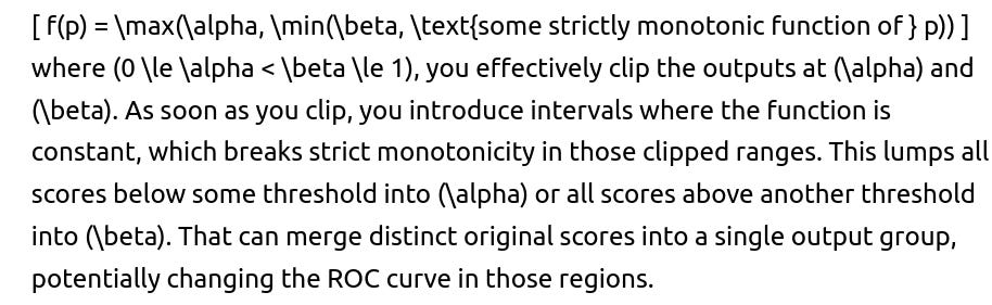
For instance, if your model sometimes outputs very high probabilities of fraud (like 0.99 or 1.0), but you clip them at 0.95 to meet some rule, then all original scores (\ge 0.95) map to exactly 0.95. This collapses a region of the distribution, losing the fine ranking among extremely suspicious cases. This can shift how TPR and FPR evolve in that upper region, slightly altering the ROC curve. In practice, the change might be minor if only a small percentage of data points fall into that clipped range. Still, one should be aware that partial clipping can alter the ranking near the extremes.
If we train a model using a loss function that is invariant to monotonic transformations, does it imply the final model’s probability outputs are also invariant?
Not necessarily. If the loss function only depends on the rank ordering (like a pairwise ranking loss used in certain learning-to-rank frameworks), the model tries to learn an ordering that separates positives from negatives well, with no strong constraints on the actual numeric scale of the outputs. This can lead to solutions that differ by a monotonic transformation in principle.
However, in practice, modern neural networks or typical classifiers often include logistic or softmax layers that explicitly produce probabilities. The training procedure (like cross-entropy) cares about both the ordering and the closeness of the model’s predicted probability to the true label. This fosters some sense of calibration. If you switch to a purely ranking-based loss, you lose some calibration impetus—so any monotonic scaling of the model’s internal scores might achieve the same rank-based loss.
Thus, the fact that a cost function or objective is rank-invariant does not mean your final numeric outputs remain unchanged under transformations in actual practice. You can end up with the same model performance in rank-based metrics while having a different numeric scale of outputs. This is often discovered post-hoc if your objective was purely about ranking.
If we observe that applying a certain function changes the area under the ROC curve slightly in practice, what might be the reason?
Possible explanations include:
Numerical Precision and Ties: Even if the function is strictly monotonic mathematically, floating-point arithmetic might cause small numerical issues. Points that were originally distinct might map to the same value due to rounding, especially in large datasets. Once they tie, the ordering among them becomes undefined, possibly shifting TPR and FPR slightly.
Implementation Details: Different software libraries might handle thresholds differently. For instance, some implementations only consider thresholds at unique values in the transformed score set. If many unique values collapse, you have fewer threshold points to evaluate, which can shift the curve interpolation.
Edge Cases at 0 or 1: If your transformation near the extremes somehow causes many values to bunch at 0 or 1, the shape of the curve near the corners may be affected in discrete increments. For large datasets, the effect can appear as small changes in the final AUC.
Even in these situations, the difference is often minimal. In theory, strictly monotonic transformations preserve the exact rank ordering, so the ideal AUC is the same. Minor discrepancies frequently stem from how real computing systems handle large volumes of data, rounding behavior, and interpolation in the ROC curve calculation.
If our model output is a logistic function of some linear predictor, and we apply a secondary monotonic function, would that change the logistic model’s interpretability in terms of log-odds?
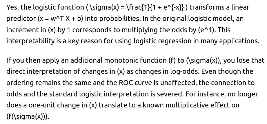
In many regulated industries (banking, insurance, healthcare), the interpretability of log-odds can be critical for compliance and for explaining decisions. Hence, even a monotonic transformation might be disallowed or heavily scrutinized for regulatory reasons because it changes how the final output is interpreted.
If we’re only interested in ranking for a top-K fraud detection scenario, does monotonicity guarantee the same top-K set of applications?
Yes, for purely rank-based selection (like “flag the top 5% highest-risk loans for manual review”), a strictly monotonic function will yield the same top-K subset, since it preserves the order of scores. The top K instances under the original scoring remain the top K under the transformed scoring because no pair of points can flip order.
The only caveat is if there are ties around the boundary of K. If you had a handful of scores that were exactly the same at the cutoff in the original scale, a transformation might break those ties differently if it expands or contracts that region in a way that merges or differentiates them. But for a large dataset with mostly distinct scores (and a strictly monotonic function preserving distinctness), the top-K set remains the same.
One potential real-world pitfall is that any slight numerical issue could break or create new ties. When working with massive data, a small fraction might see their scores change in the decimal’s last digit, which can lead to a different order among those with nearly identical scores. Practically, this might cause a small difference in the exact top-K membership, but the effect is typically minimal.
How might a strictly monotonic transformation impact the speed or efficiency of threshold searching or rank-based operations in large-scale systems?
From a purely theoretical standpoint, no difference arises in the complexity of threshold-based methods, as you still sort the data points or process them in order of their transformed scores. However, some implementation details can come into play:
Sorting Overheads: If the transform is computationally expensive to apply to each score (for example, if it involves a large table lookup or complicated function), you might incur extra overhead on very large datasets before the sorting step.
Maintaining Indices: In big data systems, you might store the original scores in certain indexes or distributed structures. A transformation might require rewriting or rebuilding those indexes, which can be significant operationally.
Mixed Precision or GPU Acceleration: In a deep learning pipeline, certain transformations might not be trivially GPU-friendly or might require additional kernels. That can change performance, though the difference might be small unless you do real-time transformations.
If the transformation is simple and cheap (like a power function or a single pass to apply (\sqrt{p})), then the overhead is minimal, and the sorting complexity remains (O(n \log n)) as before. Functionally, you still end up with an equivalently sorted list, so the threshold searching or rank-based operation is the same in complexity. It’s mostly an engineering concern rather than a mathematical or metric concern.
What if we have a multi-class problem and we apply a strictly monotonic transformation to the predicted probability for just one class? Does that preserve the ROC curve for that class vs. all others?
In a one-vs-all setting, the ROC curve for a particular class is constructed by comparing that class (positives) against all other classes (negatives). If you only transform the probability of that one class, you can alter how it relates to the other classes’ scores. For instance, suppose the classifier outputs a probability vector ((p_1, p_2, \ldots, p_K)) for a K-class problem, with (\sum_i p_i = 1). If you apply a monotonic function (f) only to (p_1), you no longer have a valid probability distribution in the typical sense (the sum might not be 1), and the relative ordering of (p_1) vs. (p_2) might change for some points.
Hence, if you compute a one-vs-all ROC for class 1 using “Is (p_1 > \text{threshold}?)” as the criterion, the ordering of (p_1) across instances can still remain the same if you apply a strictly increasing function to all (p_1) values. But if the rest of the probabilities remain in their original scale, you might inadvertently alter how you choose the “predicted class” if your inference process picks the argmax.
To preserve the typical multi-class logic and the sum-to-one property, you’d have to apply transformations that keep the distribution intact, like temperature scaling in softmax, which is globally monotonic in terms of the logits. Applying a monotonic transformation to just one class probability in isolation might cause an inconsistent set of probabilities for the multi-class system. So for multi-class tasks, transformations are more nuanced if you want to maintain consistent probability distributions and typical inference rules.
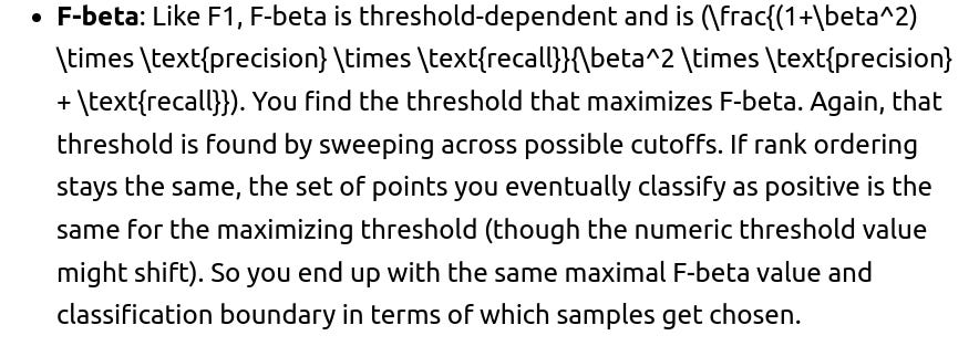
If a data scientist argues that the ROC curve is misleading in class-imbalanced tasks and insists on focusing on metrics like Weighted Accuracy or F-beta scores, does monotonic transformation preserve those metrics?
Weighted Accuracy: Usually computed as (\alpha \times \text{Accuracy on positives} + (1-\alpha) \times \text{Accuracy on negatives}), or something similar. If you search for an optimal threshold that balances these accuracies, the best threshold still depends on the rank ordering. A strictly monotonic transformation preserves that rank order, so the best threshold that maximizes Weighted Accuracy in the new scale is the same set of data points that get predicted as positive. You might have to recast the numeric threshold, but the selection of positives vs. negatives remains the same. Hence, the maximum Weighted Accuracy and how it’s achieved do not change.

In both these metrics, the final performance in terms of the confusion matrix does not change under a strictly monotonic transformation, as you can still recover the same classification boundary for each potential threshold.
What if we apply a non-strictly increasing function, such as a function that is allowed to be flat for entire intervals, but does not actually invert the order for any pair of points?
A function that is non-strictly (i.e., weakly) increasing can remain the same or constant in some segments but never decrease. In that scenario, you do not create a direct inversion. However, you do create lumps of scores that become the same value where the function is constant. For example, if a group of original scores from 0.2 to 0.3 all map to 0.5. Now these distinct original scores become identical in the transformed space. The net effect on the ROC curve depends on how those lumps contained positive vs. negative instances:
All positives or all negatives: If you lump together only positives or only negatives in that region, the step in TPR or FPR that used to happen gradually still happens, but effectively becomes a single jump in the threshold sweep. The overall shape of the curve might remain the same because you merely consolidated multiple threshold points into one step.
Mixed positives and negatives: If the interval lumps together a mix, that might slightly alter the intermediate threshold points in the ROC curve. Instead of being able to separate those positives from those negatives within that range, you see them as one big block. Depending on how the ROC algorithm enumerates unique scores and thresholds, it could merge multiple points on the curve into a smaller set of transitions. The final extremes (0 or 1 thresholds) remain the same, but the intermediate steps in the ROC curve can shift.
Consequently, a weakly increasing function can, in subtle ways, modify the intermediate shape of the ROC curve. Usually, the overall AUC might remain very similar, but you can lose resolution in the curve. The biggest effect is typically in how thresholds are enumerated, condensing multiple potential thresholds into one.
Are there cases in which a model’s post-processing step intentionally changes the ROC curve to improve certain operational characteristics?
Yes. Sometimes an organization intentionally modifies the score distribution to, for example, reduce false positives in a specific range. A typical approach might be:
Identify a region of moderately high scores that leads to too many false positives.
Transform that region downward in a controlled manner while leaving other regions mostly intact (like a partial flattening or re-scaling).
This could reorder some points or merge them, causing a partial improvement in the operating points most relevant to the business. However, it usually comes at a trade-off in other regions or metrics. Indeed, this is exactly what you do when you manipulate the shape of the curve to fit your cost preferences. You might see an improvement in TPR-FPR performance for thresholds near that manipulated range, but you could degrade or shift performance in other threshold ranges. Such a “targeted” approach is fundamentally not strictly monotonic over the entire interval. It is more of a piecewise transformation that can reorder points within the manipulated region, and thus it can reshape the ROC curve.
If we do an ensemble by averaging the outputs of multiple models and then apply a strictly monotonic transformation, is there any scenario that could change the combined ROC curve drastically?

However, you need to consider if the averaging step introduced any ties or subtle changes in ordering relative to each model’s outputs. Typically, averaging is a well-defined continuous function that preserves the rank among points if the sum of the original scores is strictly different across points. But if multiple data points had sums that were almost identical, rounding might produce ties. A subsequent monotonic transformation can’t break those ties consistently if they all map to a single value. So you might see small changes in the way thresholds are enumerated. Usually, it’s minor, but it can alter the ROC curve in discrete steps.
In general, though, if the ensemble output is distinct for each sample (no exact ties) and you apply a strictly increasing function, the ROC curve is stable. The only cause of any difference would be floating-point artifacts or tie merges.
Are there any nuances when using threshold calibration, like with CalibratedClassifierCV in scikit-learn, that might appear to change the ROC curve if we look at intermediate thresholds?
CalibratedClassifierCV often applies a calibration method, such as sigmoid (Platt scaling) or isotonic regression, to convert raw decision function outputs into probabilities. This calibration is learned on a hold-out set or via cross-validation. Because it enforces a monotonic mapping to preserve order among data points, the overall ranking does not typically change, so the ultimate ROC curve for the final predictions remains consistent with the raw decision function’s ROC curve in broad strokes.
However, you can see small differences at threshold points that are near the calibration function’s bending or flat segments. For instance, isotonic regression might flatten certain intervals that are mapped to the same probability. When enumerating unique thresholds from that set, you can see fewer distinct threshold cuts, potentially leading to a slightly different shape in the ROC curve. Typically, the area under the curve remains the same or extremely close, but the actual stepwise path can look somewhat different if you zoom in on specific thresholds.
Could a logistic transform (like applying the logit function to probabilities) preserve the ROC curve?

However, at the boundaries (p=0) or (p=1), the logit function is not defined for exactly 0 or 1. In a real model, you might get probabilities extremely close to 0 or 1 but not exactly. If some points do produce an exact 0 or 1, you must handle them carefully. Usually, we clamp them to a small (\epsilon) or (1-\epsilon). That can potentially cause some minor changes if you clamp multiple points to the same boundary. Still, for most practical data, you rarely see a massive wave of exact 0 or 1 outputs from a well-trained classifier, so the effect is often negligible. Mathematically, away from those boundaries, logit is strictly increasing, so it preserves rank ordering and the resulting ROC curve.
If the data scientist only tested the AUC after the transformation and found it was “the same,” does that guarantee the entire ROC curve is unchanged?
Measuring the AUC is a summary statistic, essentially the integral under the ROC curve. If the AUC remains the same, it strongly suggests the rank ordering is preserved. However, in a rare edge case, two different ROC curves can have the same AUC but differ slightly in shape.
Consider:
Loss of resolution: A function might flatten certain intervals, merging some threshold points. The curve might shift in those intervals but still integrate to the same overall area. This scenario is unlikely if you are dealing with a purely strictly increasing transformation, but with partial flattening, you might get some minor shape differences that do not significantly change the total area under the curve.
Discrete interpolation: Depending on how the software calculates the area (trapezoidal rule, for instance), you might see the same final AUC but slightly different TPR-FPR points if the intermediate thresholds were enumerated differently.
So having the same AUC is a strong indicator that your transformation did not meaningfully reorder the scores, but if you want to be absolutely certain, it’s best to compare the actual (TPR, FPR) coordinates or check if the transformation is strictly monotonic. In standard continuous practice, if the transformation is strictly monotonic, the entire ROC curve, including intermediate threshold points, should remain effectively identical.
If I want to interpret the model output as “log-odds,” is it enough that the transformation is strictly monotonic?

So if interpretability in terms of log-odds is critical—common in logistic regression for regulated or scientific contexts—you must either keep the logistic output or apply transformations that still allow an invertible link back to log-odds (e.g., a simple scaling or shifting might still be re-interpretable as log-odds up to a constant factor).
If we only evaluate the model’s performance at a single operating threshold (e.g., 0.5 for a binary classifier), can a strictly monotonic transformation change the classification results at that threshold?
Yes. A strictly monotonic transformation that changes the numeric values can cause some scores originally above 0.5 to move below it, and vice versa, depending on how the function behaves around that specific region. For example, if your transformation is (\sqrt{p}), then an original score of 0.36 is mapped to 0.6, which crosses the 0.5 boundary in the opposite direction from the original perspective. So if you are locked to a threshold of 0.5 in the transformed scale, you can flip which instances are considered positive.
The key is that the threshold is not automatically re-aligned with the original 0.5. If you want the same classification decisions as the original scale at your chosen operating point, you need to find the corresponding transformed threshold that yields the same set of positives. The transformation itself does not guarantee that the numeric value “0.5” in the new scale corresponds to the same classification boundary.
Hence, if your usage scenario depends heavily on applying the same numeric threshold, a monotonic transformation can still cause changes in which instances cross that threshold. That’s why threshold-based decisions might require re-mapping or re-tuning of the threshold after a transformation.
If a regulatory requirement mandates that the model output must always be at least 0.05 for any fraud probability, does that forcibly alter the ROC curve?
If you forcibly shift all predicted scores below 0.05 up to 0.05, you are introducing a constant segment in the range [0, 0.05). For any original (p) that was less than 0.05, you assign 0.05. This lumps all such scores into a single value, 0.05, losing their relative order. If some of those instances were positives and some negatives, you can no longer separate them by thresholding in that region.
The net effect is that any threshold below 0.05 is meaningless (since no predictions are below 0.05 now), and everything in [0, 0.05) is effectively the same score. This can change the intermediate steps of the ROC curve. At a threshold just below 0.05, all data in that group gets labeled positive or negative at once rather than transitioning gradually. The shape of the ROC curve in that area can shift. If only a small fraction of data originally fell below 0.05, the impact might be small, but it’s still a genuine alteration of the ranking in that region.
In real regulatory contexts, to preserve rank-based metrics as closely as possible, you might want to apply a more nuanced monotonic approach (like smoothing near 0.05) rather than a hard clip, so you can maintain a partial ordering. But that could still violate the strict requirement to never output below 0.05. So there’s an inherent trade-off: meeting the regulatory numeric requirement can degrade the fidelity of the ROC curve, especially at low threshold ranges.
How can a data scientist manage the tension between wanting to preserve the ROC curve (ranking) and wanting to produce well-calibrated probabilities for real-world use?
Commonly, you do the following steps:
Train Your Model Normally: Obtain raw prediction scores or probabilities from a classifier (like logistic regression, random forest, or neural network).
Evaluate Ranking Metrics: Check ROC AUC, PR AUC, or other rank-based metrics to ensure the model discriminates well between fraud and non-fraud.
Apply a Calibration Procedure: Use isotonic regression, Platt scaling, temperature scaling, or other monotonic methods to map raw scores to well-calibrated probabilities. Since these methods are monotonic, the underlying rank order remains unchanged, so your ROC AUC is effectively preserved.
Check the Resulting Calibration: Examine calibration plots (reliability diagrams) and compute the Brier score or expected calibration error to confirm that the post-processing is indeed improving calibration.
Validate Thresholds: After calibration, re-tune or re-select your thresholds for operational usage. Even though the ROC does not change, the numeric threshold that corresponds to a certain TPR or FPR might shift. Ensure your business or policy threshold is aligned with the new scale.
This approach lets you maintain the ranking performance and also provide probabilities that reflect real-world likelihoods as closely as possible.
If we suspect the model output was not in the range [0,1] to begin with, and we apply a monotonic function to map it into [0,1], does that have any pitfalls for the ROC?
You might encounter:
Large or Negative Values: Many classifier scores are unbounded (e.g., SVM decision function can yield negative or positive real numbers). You might try a transform such as the logistic function ( \sigma(x) ) to squash the range into (0,1). That transformation is strictly increasing in (x) so it preserves ordering. Mathematically, it does not damage the ROC ranking. But at the extremes, large positive or large negative values might compress significantly, merging wide ranges of raw outputs into near-0 or near-1 probabilities. This can lead to lumps in the distribution.
Ties from Extreme Compression: If many data points produce very large absolute value scores, the logistic function might map them all extremely close to 0 or 1, tying them numerically in floating-point representation. This lumps them together for thresholding. The net effect can be to reduce the granularity in certain ranges, which might cause small changes in the discrete steps of the computed ROC.
Nevertheless, from a strict ordering perspective, so long as ( \sigma(x) ) is monotonic, the theoretical ROC curve shape remains the same in the continuum. Numerically, lumps or ties can slightly alter the stepwise curve if large portions of data are saturated at near-0 or near-1 outputs.
How might domain-specific transformations (e.g., domain knowledge that certain feature relationships can shift probabilities) interact with the desire to preserve the ROC curve?
Domain experts might say, “Given these business rules or insights, any score below 0.2 should be lowered even further to near 0, because we suspect a strong reason that these are almost certainly not fraud.” This approach can be a partial re-mapping of the score distribution. If done in a manner that does not preserve the strict ranking (for example, if you move a subset of 0.15–0.20 down to 0.05 while leaving 0.10 scores where they are), you reorder some pairs, potentially altering the ROC curve.
In practice, domain adjustments often come from important external knowledge, so sometimes you accept the possible minor or major change in the ROC curve to integrate specialized constraints. You then re-check all your metrics. Alternatively, you can incorporate domain knowledge earlier in the model training or feature engineering pipeline. That might produce a model whose raw output already captures the domain constraints, avoiding the need for post-hoc transformations that break monotonicity.
In a distributed system where different shards might apply slightly different transformations, can this cause the global ROC curve to shift when predictions are combined?
If each shard is applying a strictly monotonic transformation but with different parameters (e.g., slightly different scaling or offsets), the local ordering within each shard is preserved. However, the relative ordering across shards can become inconsistent if the transformations do not align. For instance, a score of 0.6 in shard A might be “truly” higher or lower in the original scale than a 0.6 in shard B, but now they appear the same after transformation. Or if the transformations differ enough, a score from shard A that was originally lower might map to a higher value than a score from shard B.
When combining these predictions globally, you might lose the consistent global rank ordering. The global dataset’s ROC curve could then shift because the final merged distribution no longer respects the original order across all samples. A solution is to coordinate transformations or calibrations so that all shards share a uniform monotonic mapping. Then the combined set of predictions from all shards can be compared fairly.
What if the transformation is partially data-driven, such as applying a percentile-based rank transformation? Could that preserve the ROC curve?
A rank transformation that replaces each score by its empirical percentile in the dataset is effectively a strictly increasing mapping in a discrete sense: the lowest score becomes near 0, the highest becomes near 1, and every intermediate score takes a percentile in between. Since this transformation is monotonically increasing with respect to the original scores, it preserves the ordering exactly in an ideal sense. The ROC curve remains identical.
However, with finite data, there might be many ties or identical scores, so the empirical rank approach might assign the same percentile to multiple samples. This lumps them together, but it does not invert any ordering—it just merges them. Therefore, the final shape of the ROC curve in principle should remain the same, though you might see fewer threshold points if many samples share the same percentile rank. The AUC and major shape typically remain unaffected. This approach (rank-based transformation) is sometimes used to standardize scores for interpretability or fairness, ensuring that a fraction (q) of scores always lie below threshold (q). As an ordering-based approach, it leaves the main rank-based metrics intact.
If a candidate confuses “strictly monotonic” with “linear,” how would you clarify the difference in the context of ROC curves?
Strictly Monotonic means for any two points (p_i < p_j), we have (f(p_i) < f(p_j)). The function could be curved, piecewise linear, exponential, logarithmic, or any shape as long as it never decreases or flattens entirely over an interval.
Linear is a special case of monotonic function where (f(p) = a \times p + b). Linear transformations are indeed monotonic as long as (a > 0). But monotonicity is a broader concept that encompasses many non-linear shapes.


For ROC curves, the essential property is the strict ordering. Linear is just one easy-to-visualize example. But any function (exponential, power, logistic, rank-based, etc.) that preserves ordering—strictly increasing—does not alter the ROC curve.
It’s important in an interview to emphasize that monotonic transformations include a wide class of functions, not just linear scaling.