
ML Interview Q Series: Saddle Points vs Local Minima: Challenges in Neural Network Gradient Optimization
📚 Browse the full ML Interview series here.
Saddle Points vs Local Minima: In training a deep neural network, what is a saddle point and why can it be problematic for gradient-based methods? Contrast saddle points with local minima in terms of their effect on gradients and the training dynamics.
Saddle Points and Their Significance
A saddle point in the context of training a deep neural network is a point in the parameter space where the gradient of the loss function is zero (or very close to zero), but unlike a local minimum, it is not a point of overall "downward" curvature in all directions. Instead, a saddle point is where the loss surface curves upward in some directions and downward (or flat) in others. In mathematical terms, if we consider a point in a high-dimensional weight space where the gradient vector is zero, the Hessian matrix (second derivatives) of the loss function might have both positive and negative eigenvalues (indicating directions of local maxima and local minima), making it a saddle.
Because modern neural networks often have extremely high-dimensional parameter spaces, saddle points turn out to be much more prevalent than true local minima. This prevalence arises in large dimensions from the combinatorial interplay of positive, negative, or zero curvature across different directions in weight space.
Why Saddle Points Can Be Problematic
Saddle points can cause extremely flat or ambiguous regions of the loss landscape, where the gradient is small in magnitude. Gradient-based methods, such as plain stochastic gradient descent, may take a long time to escape these regions because the updates might become very small and inefficient at moving the parameters toward better regions of the loss surface. This extended slowdown in training can be mistaken for convergence to a local minimum, even though it is merely a plateau or region of near-zero gradient.
In contrast, a local minimum implies that in every direction around that point in parameter space, the curvature is non-negative (the Hessian has no negative eigenvalues). In a local minimum, you are at least guaranteed that small movements in any direction will not decrease the training loss significantly. With a saddle point, there are directions you can move that will lower the loss, but the gradient-based method might struggle if the gradient is too flat or if there is a high level of curvature in conflicting directions.
Training Dynamics Differences
When a model’s parameters are near a local minimum, you often see stable or slowly improving training metrics (loss or accuracy). While that might not necessarily be the global optimum, it is typically at least a stable solution in the sense that small perturbations in the parameters do not yield drastically lower loss.
Saddle points, however, can temporarily give the illusion of a local minimum because the gradient can become extremely small if the landscape is almost “flat” in many directions. But if one finds the right direction, the loss may still go down. Thus, a saddle can hinder optimization because the optimizer sees negligible gradients, making it appear stuck, even though there exist directions that lead to further decreases in loss. Modern practices such as using momentum (e.g., in SGD with momentum) or adaptive methods (e.g., Adam) can help push the optimizer out of these regions.
How They Affect Gradients
Local Minima: The gradient is zero or near zero, but the Hessian is non-negative in all directions. Small perturbations won’t help you move to a lower loss.
Saddle Points: The gradient is zero or near zero, but at least one direction has negative curvature (the Hessian has both positive and negative eigenvalues). That means you can still descend further in those directions, but first you must “escape” the region of small gradients.
Saddle Points vs Local Minima in Real-World Neural Networks
In practice, especially in very deep networks:
It is believed most “flat” stationary regions that slow down training are saddle-like, not strictly local minima.
Non-convex optimization in neural networks is often more about escaping saddles and plateaus than about avoiding high-value local minima.
Empirical observations suggest that local minima in high-dimensional settings (especially if the network is sufficiently large) are often “good enough” minima for the model to generalize reasonably.
What Are Some Concrete Indicators of Being in a Saddle Point Region?
One practical sign is that training loss stagnates for many iterations, but if you inspect the Hessian or approximate second-order information, you might discover that there exist directions in which the gradient or the curvature is still negative. Another sign is that using momentum or adaptive learning rate can suddenly cause the loss to drop after a plateau, indicating you were actually stuck in a saddle region rather than at a true minimum.
Could Noise or Stochasticity in the Gradients Help?
Yes. Stochastic gradient descent (SGD), by virtue of its mini-batch randomness, sometimes “shakes” the parameters out of saddle points. In exact gradient descent (with full-batch and no noise), a saddle could trap the optimization for a long time. The injection of noise can help the parameter updates find negative curvature directions.
Are Saddle Points Always Bad?
They are mostly undesirable for training speed because they slow down progress. However, in some situations, being near a saddle point is not inherently harmful if the plateau eventually leads to a region that is also “close” to a good local minimum. If the main priority is to keep training time short, though, you prefer to navigate out of saddles quickly.
How Do We Detect or Diagnose Saddle Points vs Local Minima in Practice?
One approach is to look at the Hessian or an approximation of it. For large neural networks, computing or storing the Hessian is often not practical. Instead, we can estimate key eigenvalues of the Hessian through efficient matrix-free approaches (e.g., using power iteration on the Hessian-vector product). If we observe negative eigenvalues, that indicates a saddle. Alternatively, we can measure the gradient norm over several directions or the variance of the gradient across mini-batches. A near-zero gradient norm with evidence of negative curvature strongly suggests a saddle.
Strategies for Escaping Saddle Points
Use Momentum: Traditional SGD can be slow in flat plateaus. Momentum accumulates velocity and can push through small gradient regions.
Adaptive Methods: Optimizers like Adam, RMSProp, or Adagrad adapt the learning rate for each parameter. They can sometimes “amplify” small gradients in certain directions, helping escape saddle plateaus.
Learning Rate Scheduling: Adjusting the learning rate can sometimes jolt training out of stagnation. Too small a learning rate might keep you stuck.
Batch Normalization and Other Architectural Choices: Certain techniques in network design can reduce pathological curvature, making it less likely to get stuck in extended saddle regions.
Second-Order Methods or Quasi-Second-Order Methods: While computationally expensive, methods like Natural Gradient or approximations with limited-memory BFGS can incorporate curvature information to escape saddles more efficiently.
Example Code Snippet for Checking Gradient Norms
Below is a tiny demonstration in Python (PyTorch) showing how one might track gradient norms during training to detect potential saddle-like behavior. (This snippet is simplistic for illustration.)
import torch
import torch.nn as nn
import torch.optim as optim

# A simple feedforward network
model = nn.Sequential(
    nn.Linear(10, 20),
    nn.ReLU(),
    nn.Linear(20, 2)
)

criterion = nn.CrossEntropyLoss()
optimizer = optim.SGD(model.parameters(), lr=0.01, momentum=0.9)

# Dummy data
inputs = torch.randn(32, 10)
labels = torch.randint(0, 2, (32,))

for epoch in range(100):
    optimizer.zero_grad()
    outputs = model(inputs)
    loss = criterion(outputs, labels)
    loss.backward()

    # Check gradient norm
    total_grad_norm = 0.0
    for p in model.parameters():
        if p.grad is not None:
            param_norm = p.grad.data.norm(2)
            total_grad_norm += param_norm.item() ** 2
    total_grad_norm = total_grad_norm ** 0.5

    # Print for debugging
    print(f"Epoch {epoch}, Loss = {loss.item():.4f}, GradNorm = {total_grad_norm:.6f}")

    optimizer.step()
If you notice the loss not improving but the gradient norm remains near zero for multiple epochs, there is a possibility of a saddle or a very flat region.
What If a Model Appears Stuck Despite Large Gradient Norm?
That scenario can happen if the direction of the gradient changes rapidly from batch to batch (e.g., if the loss surface is highly non-smooth or ill-conditioned). This is more of a gradient variance or conditioning problem rather than a saddle, so the remedy might involve adjusting the learning rate or applying gradient clipping, among other techniques.
Could We Mistake a Local Minima for a Saddle Point or Vice Versa?
Yes. Without analyzing higher-order curvature or thoroughly searching the parameter space, it can be challenging to definitively categorize a stationary point. However, in high dimensions, actual local minima that trap the network with high loss are considered relatively rare; more common are broad, flat areas in which the model can still descend if it finds the right direction. Thus, many times when training stalls, it is more likely a saddle or plateau rather than a genuine local minimum.
Additional Subtlety: Plateaus
A plateau is a region of near-constant loss without significant gradient changes. It can be caused by saddle-like geometry or simply by layers saturating (for instance, with certain activation functions). Regardless of the underlying cause, the effect is that training slows drastically. Techniques like reducing the learning rate, adding skip connections, or employing activation functions less prone to saturation might help mitigate these plateaus.
Potential Follow-up Question: How Does High Dimensionality Contribute to a Proliferation of Saddle Points?
In high dimensions, the random assignment of eigenvalues in the Hessian across different directions can produce many directions of negative curvature, many directions of positive curvature, and some near-zero curvature directions. This high-dimensional geometry makes it statistically far more probable to find points that act like saddles. In contrast, in low-dimensional problems, local minima and maxima are easier to locate or characterize.
Potential Follow-up Question: Why Might Flat Minima Sometimes Generalize Better?
A separate (but related) line of research notes that “flat” minima often correspond to better generalization properties. The rationale is that if a minimum is flat, the model’s parameters are less sensitive to small perturbations, indicating it has found a stable solution that generalizes better. However, being “flat” does not necessarily mean it’s a saddle; it can also be a flat local minimum. The question is whether that flatness is primarily in negative directions (saddle-like) or if it’s truly a benign wide basin.
Potential Follow-up Question: How Can We Use Techniques Like Entropy-SGD to Escape Saddle Points?
Entropy-SGD and related methods introduce noise or regularization forces that encourage the parameters to explore a region of the loss surface rather than settling into a single point. That exploration can help discover negative-curvature directions that lead away from saddles. By sampling from a local region of parameter space, the model effectively does a more global search, making it less prone to getting stuck in a narrow saddle.
Potential Follow-up Question: Could Clamping or Weight Decay Influence Saddle Points?
Yes. Clamping or weight decay effectively restricts the parameter values or encourages them to remain small. This might reduce the degrees of freedom in which negative curvature can become severe. While these techniques alone do not guarantee escaping saddles, they might simplify the optimization geometry enough to avoid extremely degenerate cases.
Potential Follow-up Question: Does the Sign of the Gradient Alone Indicate a Saddle?
Not definitively. A zero or near-zero gradient is necessary but not sufficient for identifying a saddle point. The key difference from a local minimum is the presence of negative curvature in at least one direction. A purely gradient-based approach might not reveal that direction unless you look at second-order derivatives (like the Hessian) or use an optimizer that implicitly leverages curvature (e.g., quasi-Newton methods).
Potential Follow-up Question: Could Over-Parameterization Make the Loss Landscape Easier?
In modern deep learning, the network is often heavily over-parameterized. Empirically, it appears that while there are many local minima, most are relatively low-loss or “good.” This can make it easier for an optimizer to eventually find a region of good performance. However, saddle points still appear all over the high-dimensional surface, so the training can pass through a series of them, occasionally slowing down but rarely staying stuck forever, especially when using best practices (e.g., momentum, weight initialization, etc.).
Potential Follow-up Question: How Do We Distinguish Between a Global Minimum and a Local Minimum?
In general, for non-convex problems like deep neural networks, it’s computationally intractable to verify that a local minimum is also global. One would have to search the entire parameter space. However, with large neural networks, the existence of multiple global minima that achieve near-zero training loss is common (especially if the dataset is not excessively large). Distinguishing local vs global is less relevant in practice; we typically settle for “good enough” local minima with acceptable training and validation loss.
Potential Follow-up Question: If Most Stationary Points in Deep Networks Are Saddles, Should We Worry?
Modern practices (e.g., large batch sizes or moderate batch sizes, momentum, high learning rates with warm restarts, etc.) usually allow optimizers to traverse these saddle regions reasonably well. Indeed, the success of deep learning in real-world tasks suggests that while saddle points exist, they usually do not permanently prevent convergence to a useful solution. The bigger worry is the efficiency of training rather than the possibility of being stuck forever.
Potential Follow-up Question: Is a Saddle Point the Same as a Plateau?
A saddle point can be part of a plateau. Sometimes you see large plateaus that occur because the gradient is near-zero in many directions (a type of extended saddle). In any case, the geometry is that one or more directions allow further descent, but the gradient-based update might be too small. A plateau can also occur if the model has saturated activation functions or other issues. Both phenomena slow training, but strictly speaking, a saddle point is about curvature, while a plateau is about the gradient being near zero over an extended region.
Potential Follow-up Question: Does Weight Initialization Affect Getting Stuck in Saddles vs Local Minima?
Absolutely. Weight initialization can determine the early trajectory through parameter space. Good initialization strategies (e.g., Xavier or Kaiming) reduce the likelihood of saturating or quickly dropping into a tricky saddle from which it’s hard to escape. However, even with careful initialization, as the network trains, it may still encounter saddles. Hence, initialization is more about ensuring that training begins in a region with a healthy gradient signal.
Potential Follow-up Question: What are Some Theoretical Results About Saddles in Deep Networks?
Researchers have shown that in high-dimensional landscapes typical of deep networks, certain favorable geometric properties arise:
Most local minima tend to have good or near-global performance.
True high-loss local minima are rare.
Many stationary points that are high-loss are saddles instead of local minima.
This perspective helps explain why standard gradient-based optimization often performs well in practice, despite the non-convexity.
Potential Follow-up Question: How Could One Illustrate a Saddle in 2D vs a Local Minima?
In two dimensions, you can depict a saddle as a hyperbolic shape (like a Pringle chip shape), sloping downward in one direction but upward in the perpendicular direction. A local minimum in 2D looks more like a bowl. In high dimensions, the concept generalizes: a saddle is where the Hessian has both positive and negative eigenvalues, a local minimum is where the Hessian has only non-negative eigenvalues.
Potential Follow-up Question: If We Perform Full-Batch Gradient Descent in a Setting Without Regularization, Are We More or Less Likely to Get Stuck in Saddles?
Full-batch gradient descent, without the “noise” from mini-batches, can in theory get stuck at strict saddle points more easily. Mini-batch methods add a certain amount of randomness that can help jostle the parameters out of saddles. Regularization (like dropout or weight decay) also changes the loss landscape, possibly altering or smoothing out certain saddles. Thus, ironically, the noise from stochastic optimization can be beneficial.
Potential Follow-up Question: What Role Does the Learning Rate Play in Dealing with Saddle Points?
If the learning rate is too low, the parameter updates in flat regions can become so small that training effectively stalls. If the learning rate is too high, it might skip over subtle but beneficial descent directions. A carefully chosen or dynamically adaptive learning rate can help the optimizer move out of saddles. Cyclic learning rates or warm restarts can also help by periodically resetting momentum or exploring different step sizes.
Potential Follow-up Question: Is There a Link Between the Generalization Gap and the Prevalence of Saddle Points?
Not directly, though they are both influenced by the geometry of the loss surface. The generalization gap is more about how well the model’s learned parameters perform on unseen data. The prevalence of saddle points mainly affects how we navigate the training loss. However, some research suggests that solutions found in wide minima or “smooth” regions (which might be near or past saddle points) can exhibit better generalization, though it’s not purely about whether or not those points are saddles.
Potential Follow-up Question: If Neural Networks Rarely Get Trapped in Bad Local Minima, Should We Still Study Saddle Points?
Absolutely. In practice, training speed and convergence behavior are significantly affected by these saddle-like structures. Even if we ultimately converge to a good solution, we can waste large amounts of computational resources dithering around a saddle. Understanding them allows us to design better optimization methods, architectures, and initialization schemes.
Potential Follow-up Question: Could We Use Gradient Clipping to Escape a Saddle?
Gradient clipping is typically used to address exploding gradients. However, if you are in a saddle where gradients are near zero, clipping won’t necessarily help. The situation is reversed: the gradient is already too small, not too large. Other techniques (like momentum or adaptive methods) are more relevant for escaping a saddle.
Potential Follow-up Question: How Could One Modify the Loss Landscape to Reduce the Impact of Saddles?
One approach is to add auxiliary or regularizing objectives that smooth the loss landscape, reducing pathological curvature. For instance, label smoothing, mixup, or other data augmentation can alter the effective training loss in ways that may flatten out highly curved regions, potentially making saddles less severe.
Potential Follow-up Question: Do Second-Order Methods Guarantee We Skip Saddles More Efficiently?
Second-order optimizers (which exploit Hessian information) can help identify negative curvature directions and move more intelligently away from them. However, in large-scale neural networks, the computational cost (both memory and time) of a full Hessian-based method is substantial. Approximations exist (e.g., K-FAC, Shampoo, or quasi-Newton) that might help, but they still may be expensive. They do not guarantee skipping every saddle quickly, but they can be more efficient at leveraging curvature information.
Potential Follow-up Question: Could Momentum Itself Fail to Escape a Very Flat Saddle?
Yes, if the gradient remains near zero for many consecutive steps, the velocity might also remain very small, making momentum less effective. But often, real-world loss surfaces are not perfectly flat, and eventually some direction of negative curvature is found. The randomness in mini-batches and the dynamic changes in layer activations can jostle the system enough that momentum can eventually push it out.
Potential Follow-up Question: Summarize the Core Differences Between Saddle Points and Local Minima
Curvature: Local minima have non-negative curvature in all directions, whereas a saddle has at least one negative curvature direction.
Trajectory: At a local minimum, any small move in parameter space won’t improve the loss; at a saddle, there is typically a direction along which we could still improve.
Effect on Training: A local minimum might be a stable point (potentially good or bad). A saddle often appears stable initially (due to a small gradient) but can be escaped if we find the negative-curvature direction. This escape can be slow, resulting in training plateaus.
Frequency in Deep Networks: True local minima with high loss are relatively rare; saddles are plentiful, especially in high-dimensional parameter spaces.
Answer Summary: A saddle point in deep neural network training is a region where the gradient is zero but the Hessian has mixed positive and negative curvature, causing the optimization to stall temporarily. In contrast, a local minimum has non-negative curvature in all directions and truly stops descent. Saddle points can be problematic because they yield very small gradients, slowing training, yet they are not genuinely minimal in all directions. In high-dimensional neural networks, saddle points are far more common than bad local minima, so much of the difficulty in training is attributed to escaping these saddle regions. Adaptive optimizers, momentum, and the inherent stochasticity of mini-batch training all help mitigate the issue of saddles in practical deep learning scenarios.
Below are additional follow-up questions
In large-scale distributed training, how do saddle points manifest and what unique challenges arise compared to single-node training?
Saddle points can become more pronounced in large-scale distributed training if different workers or nodes converge to parameter configurations that collectively land in a flat or near-zero-gradient region of the loss. Although stochastic gradient noise from each worker can help mitigate saddle point issues, the challenge is that communication overhead might mask important updates that could steer the training out of the saddle. Additionally, as mini-batches are often large in distributed scenarios, the gradients themselves can become smoother (less noisy), which can reduce the random “jostling” needed to escape saddles.
In more detail:
Synchronizing Gradients: When using synchronous training (e.g., Parameter Server or All-Reduce), all nodes must wait for each other to complete their forward and backward passes before the next step. If a significant subset of workers encounters a near-zero gradient region, the effective global update can remain very small, prolonging the time spent in the saddle.
Asynchronous Updates: In asynchronous settings, faster workers might push updates that move out of a saddle, but slower workers can lag behind, sending updates that pull the parameters back toward the saddle. This tug-of-war can lead to unstable or zigzagging convergence.
Learning Rate Tuning: The scale of parallelization often requires adjusting the learning rate. If it is set too low, the system collectively makes tiny steps in a saddle; if too high, the combined updates might overshoot beneficial curvature directions, possibly causing divergence or oscillation.
Pitfalls: A key pitfall is incorrectly attributing the plateau to hardware or software inefficiencies (communication overhead or load imbalance) when, in fact, the real issue is the saddle-like region that slows down gradient-based progress. Debugging distributed systems can be tricky because performance metrics (e.g., throughput or GPU utilization) may mask the actual shape of the loss surface encountered by the optimizer.
Edge Case: In extremely large batch training (which is common in distributed setups), the noise level in gradients is low. While a small amount of gradient noise can help escape saddles, a drastically large batch size can dampen that effect, making the optimizer linger longer in saddle regions.
Are there any specific architectures or activation functions that are more prone to getting stuck in saddle points?
Architectures with deep layers, narrow bottlenecks, or certain activation functions that saturate (e.g., sigmoid or tanh in older networks without careful initialization) can create flat or ambiguous gradients. In particular, saturating activations like the classical sigmoid can generate near-zero gradients for inputs in certain ranges, effectively creating local plateaus that mimic saddle behavior.
Detailed aspects:
Vanishing Gradients: Sigmoid or tanh can squash large inputs into regions where their derivatives are close to zero, creating long plateaus. These plateaus act similarly to saddle regions, slowing or halting the flow of gradient information.
ReLU Networks: ReLU is less prone to saturation, but it can “turn off” neurons (outputs of zero) if parameters shift into ranges that consistently yield negative pre-activation values. While this is not strictly the same as a saddle, large swaths of inactive neurons can introduce flatness.
Residual Networks (ResNets): Residual connections partially mitigate vanishing gradients by allowing the gradient to skip layers. This is not a direct remedy for saddles, but it can lessen the severity of flat regions by preserving gradient flow.
Pitfalls: One might incorrectly assume that switching from sigmoid to ReLU eliminates all saddle-related problems. While ReLU-based networks often train more reliably, they can still encounter high-dimensional saddle effects. The improvement is that they typically exhibit more stable gradients overall.
Edge Case: In some tasks (e.g., autoencoders for certain data distributions), the saturation in sigmoids might not be detrimental if the data rarely falls into extreme ranges. However, if it does, the network can get stuck in near-zero gradient regions that mimic saddle-like slowdowns.
How do regularization methods (like dropout or batch normalization) interact with saddle points?
Regularization techniques can reshape the loss landscape, sometimes making it smoother or introducing extra noise that can facilitate escaping saddles. However, the relationship is nuanced:
Dropout: Randomly dropping neurons during training adds stochasticity to the forward pass. This randomness can reduce overfitting and introduce noise in the gradients. If a network is near a saddle, dropout might cause different subsets of neurons to fire, giving varying gradients that can nudge the optimizer out of the saddle. Nevertheless, dropout alone is no magic bullet: in especially high-dimensional saddles, the improvements might be modest.
Batch Normalization: By normalizing activations, batch normalization can stabilize gradients. This makes it less likely that certain layers will saturate or become extremely flat. At the same time, batch normalization’s reliance on batch statistics could produce smaller gradient magnitudes if the entire batch sees similar data distributions in a saddle region. While BN often helps training in practice, it is not guaranteed to eliminate saddles.
** or Weight Decay**: Weight decay shrinks parameter norms over time. In principle, if a saddle region depends on large magnitudes of certain weights, weight decay could steer the parameters away. Conversely, if you are stuck in a small-magnitude region that is still a saddle, weight decay might do little to fix that.
Pitfalls: Attributing an improvement in escaping a saddle solely to dropout or batch normalization can be misleading, as many factors (learning rate, momentum, data distribution) also matter. Overuse of certain forms of regularization might slow convergence overall, so while it might help with saddles indirectly, it could also reduce training speed.
Edge Case: In small datasets, heavy regularization can overshadow the objective signal, leading to effectively random updates that might pass through saddles quickly but also degrade final performance.
Could certain loss functions be more susceptible to saddle points, and how do we address that?
Different loss functions, especially those with large “flat” regions or abrupt changes in gradient magnitude, can exhibit more pronounced saddle-like behaviors:
Cross-Entropy vs. Mean Squared Error (MSE) for Classification: Cross-entropy typically provides stronger gradients when the predictions are wrong, helping reduce flat regions. MSE can saturate if the predictions are far off, producing small gradients that may mimic a saddle. For classification, cross-entropy is usually preferred, partly to avoid these flat zones.
Hinge Loss: Hinge loss is piecewise linear. If the margin is already satisfied (i.e., the sample is on the correct side by a comfortable margin), gradients become zero. This can create plateau regions where the network sees no incentive to update parameters, somewhat resembling saddle behavior. One way to address this is margin or misclassification-based sampling, focusing computation on the “hard” examples.
Pitfalls: Merely switching from MSE to cross-entropy in classification tasks might help escape saturating plateaus, but if the data or model architecture is extreme, saddle problems can still occur.
Edge Case: In certain regression tasks where MSE is standard, the region around an optimum might be relatively flat in some directions, especially if the problem is underdetermined (many parameter solutions yield similarly low error). This scenario can look like a saddle or plateau if the network is large.
How do second-order approximations (like limited-memory BFGS) specifically detect and navigate saddle points differently from first-order methods?
Limited-memory BFGS (L-BFGS) and related quasi-Newton methods approximate the Hessian using gradient evaluations over recent steps. They can detect negative curvature directions more directly than a simple first-order method. Specifically:
Detection: If the approximate Hessian suggests there is a direction of negative curvature, L-BFGS can propose a step that moves away from that direction more aggressively. Gradient descent alone might be too small or too disoriented in that region to make significant progress.
Navigation: Once negative curvature is recognized, the update steps in a direction that reduces the loss more effectively. By contrast, plain stochastic gradient descent (SGD) can fail to exploit that curvature unless the random mini-batch noise provides enough “push.”
Pitfalls: Storing and updating Hessian approximations in high dimensions is memory-intensive. L-BFGS tries to mitigate this by keeping only a limited history. However, for extremely large neural networks, even this can be prohibitive.
Edge Case: If the batch size is small and the gradient noise is high, L-BFGS approximations can become unstable or inaccurate, ironically making it harder to detect genuine negative curvature. Thus, quasi-Newton methods might require carefully tuned batch sizes or smoothing strategies.
What role does catastrophic forgetting in continual learning scenarios have when trying to differentiate between a saddle point and a local minimum?
In continual or incremental learning, the model is trained on sequential tasks. When returning to older tasks, it may “forget” previously learned representations if the parameters drastically shift:
Relation to Saddles: A saddle region could coincide with parameter configurations that are locally optimal for a new task but degrade performance on old tasks. The gradient for the new task might be near-zero, suggesting a stall, while the old task’s gradient is not directly taken into account if we do not revisit old data (classic catastrophic forgetting).
Local Minimum vs. Saddle: In a local minimum that is truly beneficial for both old and new tasks, we might see stable or improved performance across tasks. In a saddle, training might appear to have converged for the new task but degrade old tasks drastically. This negative curvature in “old task directions” is not actively explored if old tasks’ data are absent.
Pitfalls: Attempting to define progress or stalling purely based on the new task’s loss can obscure the presence of significant negative curvature that would improve performance on the old tasks.
Edge Case: When employing methods like Elastic Weight Consolidation (EWC) or replay buffers, the additional penalties or re-introduced old data can reveal that you were not in a true local minimum for the overall objective (all tasks), but rather stuck in a partial saddle with respect to the old tasks’ solutions.
How do optimizer hyperparameters (like momentum factor or β values in Adam) specifically influence the ability to escape a saddle?
The momentum factor or exponential decay rates for first and second moments in adaptive optimizers control how quickly past gradients influence the current update:
Momentum: A high momentum factor (close to 1.0) accumulates velocity, which can help a network break free from flat or shallow saddle regions if a consistent, albeit small, gradient is present over many updates. But if there is almost zero gradient in every direction, the momentum might not build up enough velocity.
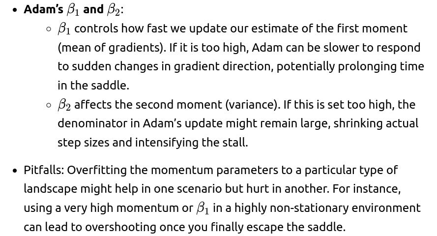
Edge Case: In extremely large, sparse parameter spaces (e.g., embedding layers for NLP tasks), adaptive methods might allocate smaller learning rates to seldom-updated parameters, intensifying the stall in directions that are rarely triggered by the data. That can keep you near a saddle if those directions are critical for escaping.
In a reinforcement learning context, where the loss is derived from rewards, do saddle points still occur and how are they addressed?
Yes. In reinforcement learning (RL), the loss function (or value function) can be highly non-stationary and non-convex. Saddle points can emerge just as in supervised settings:
Off-Policy vs. On-Policy: On-policy methods (like policy gradient) can experience large variance in gradient estimates. This noise can sometimes help escape saddles. Off-policy methods (like Q-learning with function approximation) can produce overestimates or underestimates, complicating identification of true saddle points.
Exploration: RL depends on exploration strategies (e.g., ϵϵ-greedy, policy entropy bonuses) that can inject noise into the policy updates. This often acts like mini-batch noise, pushing the optimizer away from saddles. However, if exploration is insufficient or the reward signal is sparse, the system can plateau in a saddle-like region where the policy sees little incentive to move.
Pitfalls: One might misinterpret a plateau in cumulative reward as the environment being solved or unlearnable, when in fact the agent is simply in a saddle with respect to certain state-action trajectories.
Edge Case: In environments with deceptive or sparse rewards, the entire parameter space might appear “flat” except for a few rare transitions. The agent can remain stuck in a region that yields zero gradient (no improvement in rewards), effectively a saddle from the perspective of gradient-based updates. Techniques like curiosity-driven exploration or reward shaping attempt to create stepping stones out of these plateaus.
How do curriculum learning or staged training schemes interact with saddle points?
Curriculum learning involves starting with easier tasks or subtasks and gradually increasing difficulty, guiding the optimizer through a more controlled parameter space trajectory:
Guided Trajectory: By presenting simpler tasks first, you avoid certain pathological regions of the loss landscape early in training. The parameters might move toward a region of the space where subsequent, more complex tasks lead to fewer saddles or at least shallower ones.
Pitfalls: If the curriculum transitions too quickly or abruptly, the model might be thrown into a difficult region without enough smooth gradient pathways from the simpler tasks’ parameters. This can still lead to saddle-like stalls.
Edge Case: In some tasks, even a well-designed curriculum might trap the model in a local optimum or near-flat region tailored to early subtasks. If the final tasks differ significantly, the gradual approach might not help escape a saddle that is beneficial only for earlier tasks but suboptimal for later tasks.
Does transfer learning from a pre-trained model reduce the risk of hitting saddles compared to training from scratch?
Often, yes. By starting from a pre-trained checkpoint (e.g., a model pre-trained on a large dataset), many of the raw, low-level features are already learned. This can position the model’s parameters in a region of the loss surface that is less likely to be heavily saddle-dominated:
Informed Initialization: Pre-trained weights might already be in a “valley” or broad basin of good performance for related tasks, reducing the chance of random saddle encounters. The subsequent fine-tuning is often smoother because you are adjusting high-level features rather than discovering them from scratch.
Pitfalls: If the pre-trained domain is very different from the target domain (domain mismatch), you might still encounter saddles. The advantage is less about guaranteed avoidance of saddles and more about having a feature space that’s already partially aligned with the new task.
Edge Case: If you drastically change the architecture (e.g., removing layers or adding new heads) while transferring, the newly introduced parts may face saddle issues reminiscent of training from scratch. The rest of the network might remain relatively stable, but the new layers could stall if they are large or poorly initialized.
In multi-task or multi-objective optimization, how do saddles manifest when balancing competing objectives?
In multi-task or multi-objective contexts, you have multiple losses that you often combine or trade off:
Shared Representations: The model’s shared layers must optimize for different tasks simultaneously. A saddle can arise if one task’s gradient is near zero but another task still has negative curvature directions. The net gradient across tasks might average out to near zero, creating a plateau.
GradNorm or Gradient Surgery Techniques: Methods like GradNorm or gradient surgery try to align or rescale gradients from different tasks. If one task is stuck in a saddle while others are not, gradient manipulation might break the impasse by emphasizing signals from the tasks that still have strong gradients.
Pitfalls: Overemphasizing one task’s gradient to escape a saddle can degrade performance on others, leading to a cyclical pattern of improvement for one task at the expense of the rest.
Edge Case: In certain multi-objective formulations, an actual saddle can be beneficial for one objective while detrimental to another. The optimization must find a balance or Pareto front, not just minimize a single scalar. This can complicate diagnosing whether a stall is due to a genuine saddle or a Pareto trade-off solution.
How do we handle saddle points in model compression or pruning scenarios where the network capacity is reduced?
When pruning or compressing a model, entire neurons or filters are removed, which can abruptly alter the loss landscape:
Abrupt Parameter Shifts: Pruning can move the network’s parameters into a region where many weights are zeroed out, possibly creating new saddle-like plateaus if the remaining weights must re-adapt to maintain accuracy.
Iterative Pruning: Some strategies prune gradually, alternating small pruning steps with re-training. This incremental approach can help the optimizer avoid or escape saddles introduced by large, sudden changes.
Pitfalls: A model might appear to converge to a good solution after pruning but is actually in a saddle from which it cannot significantly improve unless we reintroduce the pruned parameters (which defeats the purpose).
Edge Case: In extreme pruning (e.g., wanting a 95% reduction in parameters), the capacity is so constrained that the model effectively “flattens” the search space. Remaining parameters might quickly hit a plateau that looks like a saddle, with little chance to recover. Advanced techniques like layerwise-distillation or fine-grained structured pruning might mitigate this.
What happens if a model with discrete parameters (like a neural network with quantized weights) encounters a saddle?
In a network with quantized or otherwise discrete weights, the loss surface becomes piecewise constant or exhibits sharp transitions:
Discrete Steps: Since weights can only take on certain discrete values (e.g., 8-bit quantization), the gradient-based approach typically uses straight-through estimators or approximate gradients. This mismatch between true gradients and approximations can make saddle identification more difficult.
Plateaus Are Common: If the network is near a configuration where changing any single weight’s quantized level does not yield a beneficial outcome, we can see extended plateaus that function like saddles.
Pitfalls: One might see near-zero updates if the rounding or quantization rules push parameter changes back to the same discrete value. This can be wrongly attributed to a local minimum rather than the discrete nature of the parameter space.
Edge Case: Using fine-grained quantization schemes or gradually lowering bit precision can mitigate abrupt transitions. Yet if the final precision is extremely low, the model might remain “stuck” in a suboptimal configuration that is effectively a saddle with respect to the limited step possibilities.
In meta-learning scenarios, does the inner loop get stuck in saddles, and how does the outer loop help?
In meta-learning, we have an outer loop that updates meta-parameters and an inner loop that adapts quickly to new tasks:
Inner Loop Saddles: Each new task’s adaptation can get stuck in saddle points just like standard training. However, the timescale is shorter, and tasks are typically smaller.
Outer Loop: The meta-optimizer adjusts the model parameters (or initialization) so that the inner loop can learn effectively for future tasks. If the meta-optimizer notices that inner-loop training often stalls in saddles, it may learn an initialization that avoids regions prone to saddle issues.
Pitfalls: If the meta-outer loop is not properly tuned, it might push the initialization into a region that works for one set of tasks but fails badly for others, effectively creating new saddle-like challenges.
Edge Case: In few-shot learning, the small data per task can lead to high variance gradients in the inner loop, which might inadvertently help escape saddle points. However, if the data is too limited, it might also provide insufficient gradient signal to break free.
How could reinforcement techniques like gradient penalty or adversarial training influence saddle point dynamics?
Gradient Penalty: In some adversarial training setups (like WGAN-GP for GANs), a penalty is added to ensure gradients have a certain norm, thereby shaping the loss surface. This can sometimes smooth out sharp curvature or restrict gradient magnitude, making some saddles less severe. However, it can also flatten beneficial slopes if over-applied.
Adversarial Training: Introducing adversarial examples can significantly change the loss surface. The model is forced to learn more robust features, which might reduce the dimensionality of fragile directions in the parameter space (where negative curvature is pronounced). But adversarial training also introduces new local maxima or minima corresponding to adversarial regions.
Pitfalls: If the penalty hyperparameters are set too aggressively, it might hamper learning overall, causing everything to appear like a plateau. The network might remain near a saddle for longer simply because the penalty saturates the gradient.
Edge Case: In adversarial training, if the adversary targets specific directions in parameter space that correlate with negative curvature, it could inadvertently push the model into deeper saddle regions. Balancing these forces is a subtle aspect of robust training.
What is the relationship between mode connectivity and saddle points in neural networks?
Mode connectivity research explores paths in parameter space connecting different minima without significant rise in loss:
Continuous Paths: It is sometimes possible to connect two distinct solutions with a low-loss path. Along that path, you might traverse regions that would be saddles if you took a direct gradient-based step. However, because the path is continuous and remains at low loss, those “saddle” features are not necessarily obstacles in the broader sense.
Saddle or Bridge: A region that appears to be a saddle from a local viewpoint might be part of a smooth “bridge” between two minima when seen from a global perspective.
Pitfalls: One might mistake the ability to find a low-loss path between two minima as evidence that there are no saddles in between. In reality, the path might weave around or gently cross near-saddle regions, carefully circumventing steep negative curvature.
Edge Case: Mode connectivity typically examines solutions at scale (e.g., two well-trained networks). If the networks are in drastically different basins, the path might have to cross a region with higher loss or strong negative curvature, which is effectively a saddle zone. But advanced interpolation schemes can bypass it.
When using modern transformer architectures, do attention mechanisms reduce or exacerbate saddle issues?
Transformer architectures with multi-head self-attention are highly expressive and can learn complex dependencies:
Expressive Capacity: The high dimensionality can create numerous directions for negative curvature. However, advanced initialization strategies and layer normalization help maintain stable gradients, potentially sidestepping some saddles.
Attention Scores: The distribution of attention scores can saturate if the query-key products become very large or very small. If many heads saturate simultaneously, the model can experience near-zero gradient updates, akin to a saddle.
Pitfalls: Extremely deep transformers can develop training instabilities. If the model starts to drift into a saddle or plateau, the mismatch in attention patterns across layers can amplify or suppress gradients in unexpected ways, complicating diagnosis.
Edge Case: In certain large language model training regimes, tasks can be so broad that the model rarely fully stalls in a single saddle. Instead, partial saddles might appear for specific tokens or subsets of the data. The overall loss might still gradually improve, masking localized saddle-like stalls in certain attention heads or layers.
In evolutionary algorithms for neural network training, are saddle points still relevant?
Evolutionary or genetic algorithms do not rely on gradients but rather mutate and select neural network weights:
Indirect Relevance: Saddle points are typically a gradient-based concept. However, the fitness landscape still has regions where small mutations do not significantly improve performance. These can function similarly to saddles in the sense that random perturbations fail to find better solutions efficiently.
Hybrid Approaches: Some techniques blend gradient-based updates with evolutionary strategies, e.g., using evolution to explore parameter configurations that gradient descent might miss. This can help jump out of saddle regions.
Pitfalls: If the mutation step size is too small, the evolutionary algorithm might repeatedly sample near the saddle, failing to discover directions of improvement. If it’s too large, it could jump over beneficial basins.
Edge Case: In certain discrete architectures (like neural architecture search with evolution), the concept of a “saddle” might be replaced by “regions of low-fitness improvements.” Even if the architecture changes drastically, the phenomenon of stalling is analogous to a saddle in a continuous space.
When debugging a training run, how might you differentiate between a data pipeline issue vs. a genuine saddle point phenomenon?
Data Pipeline Issue: Common issues include data loading bottlenecks, data augmentation errors, or mismatched labels. These often manifest as sudden drops or plateaus in both training loss and throughput or the appearance that the model never “sees” a variety of examples. Analyzing CPU/GPU utilization, checking data distributions, or validating label correctness can reveal pipeline bottlenecks.
Saddle Point: When truly in a saddle, you typically observe that the model is receiving new data, but the gradient norm remains small, and the updates are minimal. Monitoring CPU/GPU usage will show that hardware is active, but the loss does not decrease.
Pitfalls: A developer might blame the optimizer for “getting stuck” when the real culprit is that half the training data is corrupted or never loaded. Conversely, someone might spend days checking the data pipeline, ignoring that the model is indeed dealing with a flat region in the loss surface.
Edge Case: In large or distributed systems, data shuffle or partial data loads can produce partial mini-batches that inadvertently push the optimizer into a saddle. It can be a combined effect of a pipeline misconfiguration and an inherent saddle phenomenon.
Are there diagnostic visualizations or statistics one can track to confirm a saddle, aside from Hessian or gradient norm?
Yes. Although Hessian-based checks are the most direct route for detecting negative curvature, there are other indicators:
Loss Landscape Visualization: In lower-dimensional settings or by using dimension-reduction techniques (like PCA on parameter snapshots), one can visualize cross-sections of the loss surface. A characteristic saddle shape might appear, with the loss dipping in some direction and rising in another.
Gradient Angle or Cosine Similarity: Track how the gradient direction changes over iterations. In a saddle, you might see the gradient direction fluctuate with little net forward progress.
Plateau Duration: A sustained plateau in the learning curve can hint at a saddle, but it could also be a local minimum or simply a region of poor gradient quality. Coupling plateau detection with small “probing” parameter perturbations can clarify if negative curvature directions exist (if the loss decreases after a small random nudge).
Pitfalls: Visualization can be misleading if you pick the wrong subspace or if the dimension reduction discards relevant directions.
Edge Case: Some losses have highly irregular surfaces that look like chaotic ridges or ravines rather than classic saddles. Simple cross-sections might fail to capture these intricacies, so the model’s “stuckness” could be mischaracterized.
How do domain shift or distribution shift events cause training to re-encounter saddle points?
When the data distribution changes between training phases or over time:
Shifted Gradients: If new data drastically changes the loss surface, the previously learned parameter region might become suboptimal, leading the model to navigate to a new region that could contain saddles.
Continual Adaptation: Models in production that face evolving user behavior might repeatedly fall into saddle-like areas if the shift is subtle enough to produce near-zero average gradient but not uniform in all directions.
Pitfalls: Engineers might see a performance drop and assume the model is stuck in a local minimum or overfitted, missing the fact that the data distribution changed. The actual fix could be data augmentation or domain adaptation, not just an optimizer tweak.
Edge Case: Rapid or extreme shifts (like a fundamental change in the user base) can produce a large gradient that moves the model quickly, bypassing small saddles. More gradual shifts can cause incremental re-training that repeatedly flirts with saddle plateaus.
How do we reconcile the phenomenon of “lottery tickets” with the presence of numerous saddle points?
The lottery ticket hypothesis suggests that large networks contain sub-networks (“winning tickets”) that can train effectively in isolation:
Saddle Evasion by Sub-Networks: A winning ticket might have an initialization that avoids the worst saddle regions even if the full network encounters them. If the sub-network’s gradient signals align more coherently, it can escape plateaus faster.
Pitfalls: Finding these sub-networks is non-trivial. If you prune or freeze weights incorrectly, you might end up with a sub-network that is still prone to saddle points.
Edge Case: Some winning tickets might rely on specific weight patterns that, while effective, still pass through saddle regions at certain steps. The advantage is that they find a route out more readily, thanks to beneficial alignments in their initial weight distribution.
Do large language models (LLMs) become less susceptible to saddles due to over-parameterization, or do they still encounter them?
LLMs are highly over-parameterized, which can mean:
Abundance of Good Minima: Over-parameterization often implies that there are many low-loss regions. The model can frequently find a path around or through saddles, especially with well-tuned optimizers and learning rate schedules.
Prevalence of Saddles: On the flip side, a vast parameter space also has countless potential saddle points. Empirically, though, large-scale training protocols (with strong momentum, sophisticated learning rate schedules, and large amounts of data) often navigate successfully through or around them.
Pitfalls: If the data is not sufficiently diverse, or if the model’s capacity is still not leveraged properly, certain narrower saddle regions might still hamper training.
Edge Case: In partial fine-tuning or few-shot scenarios, an LLM might revisit or remain stuck in a saddle if the updated parameters are a small subset (e.g., LoRA or adapter layers) that struggle to move the overall distribution out of a plateau.
In adversarial examples or model robustness contexts, can adversarial perturbations push the model parameters into saddle regions?
Adversarial attacks on inputs typically exploit certain directions in input space that produce large changes in model output:
Parameter vs. Input Space: The “saddle” concept is about the parameter space, not the input space. However, adversarial examples can cause spurious gradients that might mislead parameter updates if used in adversarial training.
Spurious Plateaus: When an adversarial training objective is added, the effective loss surface can develop new valleys or ridges. In some cases, the parameter gradients with respect to adversarial inputs can be small if the model has robustly “flattened” those directions. This could appear as a saddle for that specific portion of the data distribution.
Pitfalls: Confusing an adversarial gradient phenomenon with a saddle in the overall training objective can lead to incorrectly adjusting hyperparameters.
Edge Case: In some adversarial defenses, the model undergoes repeated adversarial data augmentation. If the distribution of adversarially perturbed inputs remains narrow, the model might get stuck in a region that is robust for that specific subset but suboptimal overall—a partial saddle scenario when viewed from the full data distribution standpoint.
Could gradient checkpointing or memory-saving techniques inadvertently affect how we escape saddles?
Gradient checkpointing trades memory for additional computation by re-computing activations during backward passes:
No Direct Impact on Curvature: These techniques do not change the loss function or the gradient itself in theory. However, numerical precision or approximate gradient schemes can cause minor differences in the update.
Pitfalls: If checkpointing is implemented incorrectly (e.g., skipping certain critical partial derivatives), it might approximate the gradient in a way that stifles small negative curvature signals. This can prolong a saddle stall.
Edge Case: In extremely large models where checkpointing is essential, the slight overhead might lead to less frequent gradient updates (due to time constraints), giving the model fewer steps to break free from a saddle within the same training budget.
Are there scenarios where a saddle might actually benefit generalization or performance?
Occasionally, near-saddle regions can coincide with “flat” areas in which the model’s parameters are insensitive to small perturbations:
Accidental Regularization: If you remain near a saddle for a while, the weights do not change drastically, potentially preventing overfitting. Once the model eventually moves out, it might have avoided the extremes of a narrower basin.
Pitfalls: This benefit is highly context-dependent and not something we intentionally seek. Prolonged stalling can waste computational resources and might never yield a better solution if the saddle is truly suboptimal.
Edge Case: In certain meta-learning or Bayesian settings, intentionally exploring regions of high uncertainty (which can appear as saddle-like plateaus) might improve exploration and lead to more robust solutions. This is not the typical “benefit” of a saddle but rather a side effect of broader exploration.