
ML Interview Q Series: Scaling Decision Tree Training Time: Insights from O(n log n) Complexity Analysis
📚 Browse the full ML Interview series here.
41. If it takes one hour to train a Decision Tree on a set of 1 million instances, roughly how long will it take to train another Decision Tree on 10 million instances?
It will likely take on the order of 10 to 12 hours. Below is an extensive, detailed explanation of the reasoning, touching upon how decision trees scale with the number of samples, what factors influence training time, and many potential follow-up questions with in-depth answers. Every subtlety and real-world consideration is explored so you can be well-prepared for rigorous Machine Learning interviews at top companies.
Understanding why the training time scales by this factor requires looking into the time complexity of decision tree training algorithms, practical considerations with large datasets, memory overhead, and subtle implementation details in frameworks like scikit-learn or other libraries. There are also common pitfalls and advanced interview questions you might face regarding how training time can vary in real-world scenarios. The discussion below aims to clarify these points comprehensively.
Training Time Complexity Intuition for Decision Trees Decision Trees typically involve recursively splitting the dataset to grow the tree. Each split tries to find an optimal partition of the data using one or more features. The time complexity often is described by an expression of the form:
A naive approach:
O(n×f×depth)
Where:
n is the number of training instances,
f is the number of features,
depth is the depth of the tree.
A more nuanced analysis:
O(n f log(n))
Because, in many implementations, the maximum depth is on the order of log(n) for balanced trees. In practice, many popular libraries will attempt to grow the tree until certain stopping criteria are met (like minimum samples per leaf or maximum depth), so the effective complexity is closer to O(n f log(n)).
In real-world terms, when n grows from 1 million to 10 million, you’re increasing the dataset size by a factor of 10. If a decision tree’s training complexity is roughly proportional to nlog(n), then going from n to 10n can multiply training time by around:


Since real systems do not always perfectly reflect this theoretical ratio (due to memory constraints, implementation details, multi-threading, etc.), a practical rule of thumb is somewhere around a factor of 10–12. This is why, if it took 1 hour on 1 million instances, we can expect ~10–12 hours for 10 million instances.
Hence, the direct short answer is that training another Decision Tree on 10 million instances would likely take about 10–12 hours, acknowledging that actual times may vary depending on the number of features, hardware, software, and other complexities in the data and the implementation.
Below are several follow-up questions that might arise in an interview, along with comprehensive, in-depth answers to help prepare you for the conversation.
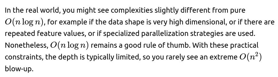
How does the depth of the decision tree affect this time complexity, and are there practical constraints that alter the theoretical O(nlogn) assumption?
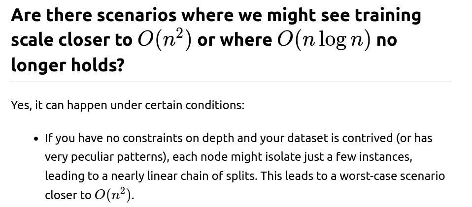
When building a decision tree, each node partition attempts to split the data along a feature threshold that yields the greatest information gain (or lowest impurity). The maximum depth of a completely unrestricted binary tree could theoretically approach n in the worst case (imagine an extremely overfitted tree that divides nearly every sample onto its own leaf). However, in practice, trees are often not grown that deep due to:
Early stopping criteria. Decision tree libraries commonly have hyperparameters such as max_depth, min_samples_split, or min_samples_leaf, which place explicit constraints on the growth. This helps avoid both overfitting and excessive computational cost.
Data distribution. Unless the features perfectly separate the samples at each node, the splits tend to reduce the dataset more or less evenly, making the depth often scale more like log(n) rather than n.
Potential pitfalls:
If you remove all constraints on depth, training time can grow unpredictably.
Imbalanced or extremely skewed data can result in deeper trees if the algorithm fails to find strong splits early on.
If you have an extremely large number of features (say tens of thousands or more) and your implementation must evaluate many split candidates exhaustively, the cost could be significantly higher. Some libraries attempt to mitigate this by sampling features or using approximate splitting strategies.
If your dataset includes many identical or near-identical feature values, the splitting process might degrade in performance because the splitting algorithm has to check many thresholds that yield the same or similar impurity reductions.

If the depth of the tree is constrained, does the training time reduce significantly?
Yes, constraining the depth has a direct impact on training time because you limit how many times you can split the data. If you set max_depth to a relatively small number, then each path from the root to a leaf has fewer nodes, and you have fewer potential split evaluations. In that sense:
When max_depth is fixed and fairly small, the training time can become closer to O(n) or O(nf), because you only do a set number of splitting operations at each level, and the number of levels is capped.
Limiting depth can make the model simpler (lower variance) but might introduce bias if the tree can no longer capture more complex patterns.
Because most real datasets have enough complexity that we want some moderate depth, the typical scenario remains something in the ballpark of O(nlogn) but with a lower constant factor. This is why big improvements in training time can be seen when you reduce max_depth from, say, 50 to 10.
How does the number of features impact training time when comparing 1 million vs. 10 million instances?
The presence of additional features (f) can multiply with the nlog(n) factor. Specifically, you might see complexity like:
O(nflog(n))
If you multiply n by 10 but keep f fixed, you primarily multiply that part of the training complexity. However, if you simultaneously increase the feature dimension f, training can become more expensive in an even more pronounced way. Many frameworks can sample features at each split (especially in random forests) to reduce complexity. Still, in a straightforward decision tree approach that checks every feature at each candidate split, increasing f can significantly increase training time.
Real-world scenarios:
In practice, if you go from 1 million to 10 million samples while also going from 100 features to 1000 features, your training time might increase by more than the pure ratio factor of nlog(n), because you’re also exploring more features for each potential split.
If your pipeline includes feature selection or dimensionality reduction, then you may keep f smaller and keep the training time more manageable.
What if we parallelize or distribute the training—would that reduce the time in a linear fashion?
Parallelization often helps, but it rarely provides a perfect linear speedup because of the overhead of data movement, synchronization, or communication among workers. Many decision tree libraries exploit parallelism by:
Splitting the data among multiple threads or processes.
Parallelizing the search for the best split at each node across different features.
Parallelizing the evaluation of multiple candidate thresholds.
However, the overhead of concurrency can lower your effective speedups. Also, if you’re using a single multicore machine, memory bandwidth can become a bottleneck when dealing with large datasets. In distributed solutions (like Spark MLlib or other big-data frameworks), you might reduce training time by scaling across many machines, but you incur inter-node communication overhead and must handle partitioning efficiently.
In short, parallelization can help you go from, say, 10–12 hours to fewer hours, but it’s not always going to be a direct factor-of-8 or factor-of-16 improvement (depending on how many cores you have). Real improvements are often less than the theoretical maximum due to communication overhead, load balancing, and memory access patterns.
Are there any practical code examples on how we might measure or approach this scaling with a toy setup?
Below is a small illustrative code snippet using scikit-learn’s DecisionTreeClassifier. Of course, this is a toy example and not truly operating on millions of data points, but it demonstrates the typical structure of training code in Python:
import numpy as np
from sklearn.tree import DecisionTreeClassifier
import time

# Toy example: we'll just simulate data
# In practice, you would load an actual dataset, e.g. from a CSV or a data pipeline
n_samples = 10_000_00  # smaller than a million for illustration
n_features = 20

# Generate random data
X = np.random.randn(n_samples, n_features)
y = np.random.randint(0, 2, size=n_samples)

# Create the Decision Tree classifier
tree_clf = DecisionTreeClassifier(max_depth=None, min_samples_split=2)

# Measure training time
start_time = time.time()
tree_clf.fit(X, y)
end_time = time.time()

print(f"Training time for {n_samples} samples: {end_time - start_time:.2f} seconds")
If you scale n_samples by a factor of 10 (while still in feasible memory limits), you would measure how the time changes. The ratio would give an empirical sense of scaling. On a typical desktop machine, you might see a time ratio somewhat in line with the nlog(n) or a little more or less, depending on overhead, memory, or parallelization.
In a real large-scale setting with 1 million or 10 million rows, you’d need enough RAM to hold the data. This quickly becomes a practical constraint. Tools like Spark ML or Dask-ML allow distributed data storage and training, but again, overhead and the complexities of distributed training come into play.
If the data has many categorical features or missing values, does it change how quickly the decision tree trains?
Categorical features. If each categorical feature is handled by one-hot encoding or some other encoding strategy, the resulting feature space grows, effectively increasing f. This can increase training time. Some implementations have specialized splits for categorical variables (grouping categories vs. searching across the entire expanded one-hot dimension). This can reduce overhead but is often not as straightforward as numeric splits.
Missing values. Some libraries (like XGBoost) have specialized logic to handle missing values in a branch-aware manner. Traditional implementations (like the standard scikit-learn DecisionTreeClassifier) typically require you to decide how to handle missing data beforehand, such as filling them with some default value or dropping incomplete rows. Each of these strategies can slightly alter how much data is available at each node, but generally, it doesn’t drastically reduce or increase the big-O complexity—though real-world overhead might go up if you do a lot of preprocessing or complicated imputation.
Is there a rule of thumb for how large a dataset can be before a single decision tree becomes infeasible to train?
In many real applications, once you get into tens or hundreds of millions of samples (and especially if you also have thousands of features), training a single decision tree on a single machine can become very slow or require more RAM than is practical. That’s one reason why:
Practitioners often switch to tree-based ensemble methods (Random Forest, Gradient Boosted Trees) that have distributed training support (e.g., Spark’s random forest, XGBoost distributed mode, LightGBM distributed mode).
Data scientists might apply subsampling to keep the dataset at a manageable size. For instance, if you have 100 million rows of data, you might randomly sample 10 million to train your tree. This approach can be quite effective if your data is fairly homogeneous and you only need a subset to capture the patterns.
A typical rule of thumb is that if you can fit the entire training dataset in memory and still train within a few hours, it’s feasible to proceed on a single machine with an optimized library. Beyond that, it might be more efficient to use distributed solutions or dimensionality and sample-size reduction strategies.
What if we used a random forest or gradient-boosted trees instead—would the time scale similarly from 1 million to 10 million?
Random forest. A random forest trains multiple decision trees on bootstrap samples of the data, often in parallel. Each tree is typically grown to maximum depth (or close to it), and features are randomly sampled at each split. The overall training time is roughly the number of trees multiplied by the time to build one tree, with some performance gains from parallelization. Hence, if each individual tree scales from 1 million to 10 million in about a factor of 10–12, then building a random forest of, say, 100 trees can scale similarly, though parallelization can reduce the total wall-clock time.
Gradient boosting. In gradient-boosted decision trees (e.g., XGBoost, LightGBM, CatBoost), you iteratively train trees, each one focusing on the residual errors of the previous ensemble. While each tree might be smaller or shallower than a full decision tree, the total number of trees is typically in the hundreds or thousands. The scaling from 1 million to 10 million is still significant but can be more optimized by specialized implementations that do histogram binning and approximate splits. They also have distributed training modes. Overall, you can still expect that going from 1 million to 10 million can increase training times by about an order of magnitude or so, with overhead depending on the library’s optimizations.
Are there ways to reduce training time when scaling up from 1 million to 10 million samples?
Subsampling. Often, a random subset of 10 million rows can produce a model of comparable quality to using the entire dataset, especially if the data is somewhat redundant. For instance, you might only use 5 million out of the 10 million rows to cut training time significantly.
Feature selection. Reducing the dimensionality of your data, either through domain knowledge or automated methods, can make training faster if you have many features with little predictive power.
Using approximate or histogram-based splits. Some modern libraries for gradient-boosted trees (e.g., XGBoost, LightGBM) build histograms of feature values rather than evaluating every possible threshold. This can drastically reduce the complexity while still offering high-quality splits.
In-memory vs. on-disk. If the dataset can be loaded in memory, the training will typically be much faster than if you must read from disk in smaller batches. So ensuring you have sufficient RAM or that you use an efficient distributed in-memory platform can help.
Parallelism and distributed training. As mentioned, using multiple cores or multiple machines can bring down wall-clock time significantly, although it does not change the total computational work by as large a factor.
Could the time be shorter than 10 hours if we are going from 1 million to 10 million rows?
While the theoretical scaling suggests 10–12 hours, real systems are complex. There can be reasons your actual training might end up faster than a naive 10× scaling:
Caching effects on smaller subsets of data might become less optimal with bigger data, but you might also see some numeric or parallel efficiency changes. Sometimes, an implementation might process data in chunked form, so going from 1 million to 10 million doesn’t necessarily multiply everything by 10 if certain overheads are amortized.
If your model is configured differently for larger data—such as a shallower max_depth or a larger min_samples_leaf—you could see training times that are more modest than a direct scale-up would suggest.
However, in many straightforward scenarios (same hyperparameters, same hardware, same library), the training time from 1 million to 10 million will not magically become less than an order-of-magnitude difference. It’s often prudent to assume near a 10× scale-up and then measure empirically.
If I have to handle 10 million data points, what memory constraints should I consider?
Memory usage can be substantial when fitting large decision trees. The data alone might take gigabytes if you have many floating-point features. Additionally, decision tree algorithms can create temporary data structures during training, particularly if you’re evaluating multiple potential split thresholds. As a rough guideline:
Each floating-point (e.g., float32) feature value for 10 million rows can take 4 bytes. So if you have 100 features, that’s 4 × 100 × 10 million = 4,000,000,000 bytes = about 4 GB just to store the raw feature matrix, ignoring overhead.
Some libraries create copies of subsets of the data or store indices for subsets as they build the tree. This can multiply the memory requirement by 2–3× or more, depending on the implementation.
If your data is stored in a data structure that is not memory-efficient, or if you keep multiple copies in memory (for example, a Pandas DataFrame plus a NumPy array plus internal data structures), the memory usage can balloon quickly.
Hence, it’s not just time but also memory that can become a bottleneck. One must ensure the hardware can handle these demands or switch to streaming/distributed solutions if memory is limited.
Could on-the-fly methods or streaming decision trees help?
Some algorithms attempt an online or streaming approach. Rather than reading the entire dataset in memory, they incrementally update the tree structure as new data arrives. Many standard libraries don’t do this by default for decision trees, but there is research and some implementations of online decision trees that can handle data in a streaming manner. These approaches can reduce memory demands and sometimes accelerate training for very large data, but might not always produce the same results as a full batch training approach.
In many real situations where data is extremely large, data scientists turn to either:
Gradient boosting frameworks that implement approximate splits or distributed training.
Random forest implementations on top of Spark or HPC clusters.
Subsampling strategies if a near-equivalent model performance can be achieved with partial data.
Summary of the main question’s short answer
Given all the above, the direct answer to the original question—“If it takes one hour to train a decision tree on 1 million instances, how long will it take on 10 million instances?”—is that you should expect around 10 times or slightly more, in the 10- to 12-hour range. The reasoning is rooted in the approximate O(nlogn) training complexity. Real-world conditions might push it higher or lower, but a rough factor of 10–12 is a good rule of thumb. You can refine that further by measuring actual training times on your specific hardware and software.
This thoroughly addresses the reasoning behind the scaling factor and the typical complexities you might encounter in practice. The follow-up questions provide a fuller picture of potential interview discussions you could have when asked about how decision tree training time grows with the dataset size, how hyperparameters and data distributions affect scaling, and possible ways to mitigate long training times.
Additional Follow-up: Is there a difference in how scikit-learn, XGBoost, and LightGBM handle large data for decision trees, and could that alter the 10× rule-of-thumb?
Yes, there are differences:
scikit-learn’s DecisionTreeClassifier. This library uses a relatively straightforward, exact splitting algorithm for each node. It evaluates all possible split thresholds for each feature. Hence, it can be slower on large datasets but is easy to understand and debug. The 10× rule-of-thumb from 1 million to 10 million is a decent estimate for scaling in scikit-learn.
XGBoost. Uses histogram-based approximate splits by default. This means it first buckets continuous feature values into discrete bins, which can significantly reduce the overhead of searching for exact thresholds. Therefore, the training might scale better or worse depending on how many bins are used and how the data is distributed. You could see a scaling factor still close to 10×, but sometimes XGBoost’s clever parallelization might yield a speedup that is more favorable than naive expectations.
LightGBM. Also histogram-based, often more aggressively so. It uses gradient-based one-sided sampling and other optimizations that reduce computational overhead. In practice, you might see that LightGBM can handle tens of millions of rows quite well, scaling in a near-linear fashion with some overhead for communication if running distributed. It might still be in the ballpark of 10× from 1 million to 10 million, but some hardware setups yield a bit less than that due to efficient parallelization.
Overall, the 10× rough scaling factor remains a good baseline for top-level conversation, but real measurements on your hardware with your specific library are always recommended.
Final Note
As soon as you see the question “It takes 1 hour on 1 million rows, how long does it take on 10 million rows?” in a technical interview, the interviewer is often testing if you understand:
The approximate O(nlogn) complexity of building a decision tree.
The notion that 10 million is 10 times 1 million, but due to the logn factor, the real scaling is somewhat more than just 10×, closer to 11–12× in many typical cases.
The practical difference between theory and real-world performance (hardware constraints, library optimizations, etc.).
Hence, about 10–12 hours is the succinct yet well-reasoned answer, but showing that you know why is crucial.
Below are additional follow-up questions
What is the effect of extremely correlated features on training time?
When features are highly correlated, you might expect that some splits effectively partition the data in almost the same way as others. In theory, having multiple very similar features means the decision tree algorithm repeatedly checks nearly redundant splits, which can slightly increase overall computation. However, in practice, most implementations still evaluate each feature (and each potential threshold) separately, so the time complexity doesn’t magically drop just because features are correlated.
Potential pitfalls and edge cases:
Even if redundant features can lead to similar splits, you don’t necessarily get a speedup because the algorithm must still compute the impurity improvement for each candidate split unless you explicitly remove or combine correlated features beforehand.
If you do feature selection or dimensionality reduction to address high correlation, you can reduce the effective number of features. This can yield a tangible speedup, especially at large scale (from 1 million to 10 million rows).
Logical conclusion:
Highly correlated features can add overhead because the decision tree doesn’t automatically skip them. In real-world systems, removing or combining them via domain knowledge or PCA-like methods can help reduce training time.
If we have real-time constraints and want to do an online update, how does that differ from typical offline training?
Typical offline training loads a fixed dataset into memory, constructs the tree in a top-down manner, and completes the process in a single pass over that data (with recursive splits). In contrast, online or incremental training aims to update the tree structure as new data arrives, without retraining from scratch.
Key considerations:
Many standard decision tree libraries (like scikit-learn’s DecisionTreeClassifier) do not support partial_fit; they assume the entire dataset is available at once.
Online decision tree algorithms (e.g., Hoeffding Trees) often approximate splits and do not revisit previous splits extensively because that would require storing and reprocessing historical data. This can reduce accuracy compared to a fully trained batch tree but allows training to scale with an ongoing data stream.
Potential pitfalls:
Memory usage might be smaller or more controlled in streaming methods, but you lose the ability to do an exact global search for the best splits across the entire dataset at once.
If you expect to handle 10 million events streaming in real time, you must ensure that the incremental approach processes data fast enough to keep up with incoming samples.
Logical conclusion:
Online or incremental updates differ fundamentally from batch training in how splits are decided and updated. For real-time systems, the design is oriented more toward sustained throughput than to the exact O(nlogn) complexities typical of offline training.
Does training a Decision Tree for multi-class classification significantly differ in time from binary classification, especially if we have many classes?
Decision trees handle multi-class classification by evaluating impurity measures (like Gini or entropy) that can be generalized to multiple classes. The steps for finding a split are still essentially the same: evaluate potential splits and measure how well they separate the classes.
Time complexity perspective:
In principle, for each candidate split, you now compute an impurity reduction over multiple classes rather than just two. That might slightly increase the arithmetic needed because you must sum or compute probabilities across multiple categories.
The difference is often not major if you have, say, under 10 classes. With extremely large numbers of classes (e.g., thousands), the cost of calculating impurity at each node can grow noticeably.
Potential pitfalls and edge cases:
If you have a huge number of classes, storing and updating class counts at each potential split can be more time-consuming and require more memory.
Some libraries optimize multi-class impurity calculations with efficient data structures or partial histograms. Others might degrade in performance significantly with many classes.
Logical conclusion:
For small to moderate class counts, multi-class vs. binary classification usually doesn’t change training time drastically, although you should anticipate some overhead. For extremely large class counts (like thousands or tens of thousands), multi-class classification can add significant overhead.
Is there a difference in training time if we use Gini impurity versus entropy as the splitting criterion?
Both Gini impurity and entropy measure how well a split separates the data into pure nodes. The difference is in the formula used:
Gini impurity tends to be simpler and slightly faster to compute in many implementations.
Entropy requires computing logarithms for each class probability.
Potential pitfalls:
The difference can be negligible in modern CPUs for smaller numbers of classes, since log operations are not prohibitively expensive.
For very large multi-class problems, the repeated use of log operations can become more expensive. Some libraries vectorize these calculations efficiently, so the gap is still small.
Logical conclusion:
Generally, Gini is marginally faster than entropy, but both scale similarly with n. You won’t see a drastic difference (like halving the training time) just by switching from entropy to Gini, but the effect can be more apparent with a massive dataset and many classes.
If we have a highly imbalanced dataset, does that change the training time or the best approach to training?
Training time perspective:
The algorithm still performs the same splitting logic, so in principle, the big-O complexity doesn’t shrink just because the classes are imbalanced. You still have to evaluate potential splits at each node.
In practice, if one class overwhelmingly dominates, some splits might be trivial or produce very similar impurity improvements. But you don’t typically see a large time reduction because the algorithm must still evaluate candidate thresholds for all features.
Best approach considerations:
You might adopt class weighting or sampling techniques (e.g., SMOTE for oversampling the minority class). These strategies can alter how the data is distributed during training, potentially reducing or increasing the effective dataset size used in each tree-building iteration.
You can also adjust min_samples_split or min_impurity_decrease to handle rare classes more effectively, but that doesn’t necessarily reduce the overall computational cost unless the parameter changes significantly reduce the depth or number of splits.
Edge cases:
If you heavily undersample the majority class, you could reduce the total dataset size and thus reduce training time, but that might harm accuracy if you remove too many majority instances.
Logical conclusion:
Imbalance primarily affects the model’s ability to detect minority classes rather than drastically altering the fundamental time complexity. If you do want to reduce training time, undersampling or other approaches might help but at potential cost to model coverage of the majority class.
What if we incorporate monotonic constraints in a tree-based model?
Monotonic constraints require that the predicted value of the model move in only one direction (non-decreasing or non-increasing) with respect to certain features. Some gradient-boosted frameworks (like XGBoost, LightGBM, CatBoost) support monotonic constraints on splits.
Training time implications:
Standard, unconstrained decision tree algorithms do not handle monotonic constraints by default. If you enforce them, the search space for valid splits is reduced, potentially lowering or increasing the overhead depending on the implementation:
On one hand, the algorithm might skip or prune splits that violate the constraint, which can reduce the candidate splits it must evaluate.
On the other hand, the internal logic to check monotonicity can add overhead if it’s done repeatedly.
Edge cases:
If multiple features have monotonic constraints, the complexity of checking or enforcing them can grow. Some libraries might implement partial constraints that are simpler to enforce, while others do a more complex search.
Logical conclusion:
Monotonic constraints can lead to simpler trees or fewer candidate splits, which might reduce training time, but it depends heavily on how the library implements them. If the library’s approach is not optimized, you might see some overhead from verifying constraints at each node. Overall, it doesn’t typically blow up training time, but it can alter it in subtle ways.
If we do partial fitting for a streaming scenario, does that change the scaling from 1 million to 10 million data points?
Partial fitting implies that you train on small batches of data iteratively. Each batch might be, for example, 10,000 rows. Over many batches, you accumulate knowledge of the entire 10 million data points without loading them all at once.
Key considerations:
A partial_fit algorithm that re-structures an entire tree from scratch for each batch can be very costly. You might see something closer to ParseError: KaTeX parse error: Expected 'EOF', got '_' at position 14: O(\text{batch_̲count} \times \…. If you have 1,000 batches of size 10,000 each, that overhead can add up.
True online decision trees (like Hoeffding Trees) update the model without fully rebuilding from scratch, so the cost per additional batch is smaller. The net effect might still scale roughly linearly with the total data size, but each incremental update is more efficient than a full batch rebuild.
Edge cases:
If the partial_fit approach is naive (i.e., it doesn’t store intermediate statistics and tries to train from scratch each time), your time can scale poorly with the total data size.
Some libraries do not implement partial_fit for regular decision trees, only for other algorithms like naive Bayes or stochastic gradient descent.
Logical conclusion:
Partial or incremental training can help with memory constraints, but the total computational effort might still scale in a similar or even more expensive way than a single-shot training, depending on how efficiently the library implements incremental updates.
How do we handle extremely large cardinality categorical features (billions of unique categories) for decision trees?
Standard decision tree splits typically require enumerating thresholds or categories. For categorical features with billions of levels:
Naive one-hot encoding is completely infeasible because it explodes the feature dimension.
Most standard libraries cannot handle that many categories directly because they typically sort unique category values or attempt a brute force approach to find the best subset of categories on each split.
Potential solutions and pitfalls:
Use hashing-based encodings (e.g., feature hashing) to map categories into a lower-dimensional space. This can reduce cardinality drastically, although collisions might degrade model quality.
Consider domain-specific grouping or embedding-based methods to cluster categories with similar outcomes before training the tree.
Libraries like LightGBM can handle some categoricals natively, but still not in the range of billions without pre-processing.
Training time implications:
If you reduce the effective dimensionality, you can keep training times more manageable. If you do not, the algorithm may spend a prohibitive amount of time evaluating splits, or it may run out of memory.
Approximate or distributed solutions might help, but the data transformation overhead can still be huge.
Logical conclusion:
Extremely large cardinalities require careful preprocessing to avoid ballooning feature space. Once you manage to reduce the cardinality effectively, the scaling from 1 million to 10 million rows can return to the typical O(nlogn) pattern for decision trees.
What if the data is stored on disk, and we cannot fit it in memory? Does chunking or memory mapping affect training time scaling from 1 million to 10 million?
If the data can’t fit in RAM and is stored on disk, you often resort to chunking, memory mapping, or distributed data frameworks:
Chunking means reading segments of data sequentially, partially building or updating the model. Traditional decision trees in scikit-learn do not natively support chunked training, so you might have to store partial information or use a specialized library.
Memory mapping (e.g., using NumPy’s memmap) can help you treat disk data as if it’s in memory, but random access can be much slower, increasing training times drastically.
Edge cases:
If the dataset is so large that you exceed the OS cache and have significant disk I/O, the training time might scale worse than 10× going from 1 million to 10 million rows because random access patterns can magnify I/O overhead.
If you’re using a distributed framework like Spark MLlib, each worker might still need to shuffle or sort partial data, so the network or disk overhead can become a bottleneck.
Logical conclusion:
Handling large data on disk often increases overhead, making the naive 10–12 hour rule-of-thumb too optimistic. Actual times might be significantly longer due to I/O bottlenecks. Chunking or distributed methods can mitigate this but come with their own overhead.
Are there potential numerical stability or floating-point precision issues that might appear at 10 million rows that wouldn’t show up at 1 million?
Training decision trees generally involves summing up counts of instances belonging to classes (for classification) or summing target values (for regression) to compute impurities or variances. At 10 million rows:
Summations might become large, but they often fit within standard 64-bit floating-point or integer types.
Some frameworks use single-precision floats for speed, which can lead to rounding issues when dealing with large sums or extremely close thresholds.
Pitfalls:
If you’re doing regression with very large target values, intermediate sums can overflow a 32-bit float. Some implementations might handle that gracefully by switching to 64-bit, but if not, you could see numerical anomalies.
For classification, especially multi-class with large counts, the probabilities used in Gini or entropy calculations might become extremely small or extremely large, but typically 64-bit floating-point can handle it.
Logical conclusion:
While uncommon, numerical precision issues can crop up at tens of millions of data points, especially in single-precision contexts. Most well-tested libraries mitigate this with double precision or robust summation strategies, but it’s a subtle concern at scale.
If the data is not i.i.d. or if we have time-series data, does that affect how we measure training time or how we scale up from 1 million to 10 million?
From a pure training time perspective, the algorithm’s complexity is still driven by how many rows and features it processes. Whether the data is i.i.d. or time-series does not fundamentally change the split search procedure.
However, real-world considerations:
For time-series data, you might enforce certain constraints (e.g., you cannot split on future data when training on past data). This can lead to specialized training flows or windowed modeling, where you only train on data up to a certain point in time.
If the data is not i.i.d. (e.g., it has correlation over time), it might produce deeper or more complex trees, depending on how the splits are discovered, but this typically doesn’t drastically alter the big-O scaling.
Edge cases:
In an online time-series approach, you might retrain or update your model daily or hourly. The total number of rows eventually grows to 10 million over time, and partial/online fitting might be used. This changes the operational perspective of training, but not the fundamental complexity if you eventually see all 10 million data points.
Logical conclusion:
Non-i.i.d. data or time-series constraints can change the way you structure your model training pipeline, but the raw computational scaling for a naive top-down tree build typically remains similar. The difference usually lies in how you chunk or sequentially feed the data rather than the algorithm’s complexity formula.
Does a distributed environment with unreliable network conditions hamper the 10× scaling factor from 1 million to 10 million?
When you distribute training across multiple nodes, you rely on network communication to aggregate statistics, share partial model information, or shuffle data:
In an ideal scenario with a high-bandwidth, low-latency network, you can see near-linear speedups with enough workers, potentially offsetting the 10× factor.
With unreliable or slow network conditions, the overhead can dominate. You might end up waiting for straggler nodes or re-sending data. This can make scaling from 1 million to 10 million worse than expected because the communication overhead scales with the data size.
Edge cases:
If one node is especially slow or if the cluster experiences random failures, training might stall or require restarts. This is especially problematic when you multiply data by 10.
Some frameworks are more resilient to partial failures, but each framework can add overhead in monitoring and synchronization tasks.
Logical conclusion:
Distributed training does not guarantee the straightforward 10× scale in time. Under unreliable conditions, you might lose much of the efficiency you hoped to gain, and actual training time might balloon. Proper cluster management and robust data partitioning strategies are crucial.
If we do dynamic feature engineering or transformations during training, does that significantly alter the scaling assumptions?
Dynamic feature engineering implies that at each stage (or node split), you might generate new features or transformations (e.g., polynomial expansions, domain-specific transformations). This is not standard in typical decision tree algorithms, which rely on a fixed set of input features.
Potential impacts on time complexity:
If you compute new transformations for each node’s subset of data, that adds overhead proportional to the number of subsets and splits. So the training time might grow more than O(nlogn), depending on how complex the transformations are.
Realistically, you might do transformations once before training, thus not changing the per-node overhead. But if your transformations depend on partial statistics from each subset, you effectively do extra computations at every level of the tree.
Edge cases:
If transformations are lightweight (like scaling or simple arithmetic), it might not massively affect runtime. If you do more advanced transformations (like deep feature extraction with a separate model), it can drastically slow training.
Logical conclusion:
Standard scaling assumptions (O(nlogn) for building a tree) assume the features are fixed. Dynamic transformations break that assumption, potentially pushing beyond the naive factor-of-10 rule when data grows from 1 million to 10 million, depending on how often transformations are computed and how expensive they are.
If we have HPC hardware with GPU acceleration, does that drastically reduce the scaling factor from 1 million to 10 million?
GPU acceleration for trees typically appears in boosted-tree frameworks (e.g., XGBoost, LightGBM, CatBoost). A single decision tree algorithm (like scikit-learn’s) might not offer GPU support in the same way.
Considerations:
On a GPU-accelerated library, you can significantly speed up the histogram-building or split-search steps, often seeing large improvements in training throughput.
Going from 1 million to 10 million points, you could see scaling that remains roughly a 10× increase in total computational work, but the absolute training time is much smaller due to the GPU.
The speedup might be sublinear with respect to the number of GPU cores due to memory transfer overhead, GPU kernel launching overhead, or the cost of reading data from host memory.
Pitfalls:
GPU memory is a fraction of typical CPU system memory. For 10 million data points, you might run out of GPU RAM if you attempt to store all features or histograms on the GPU, forcing chunking or a hybrid approach that can reduce speed gains.
Implementation details (e.g., how well the algorithm saturates GPU cores) can drastically affect real-world performance.
Logical conclusion:
GPU acceleration can shrink absolute training times. However, the ratio of time from 1 million to 10 million data points can still be around a factor of 10, unless the overhead of GPU transfers or kernel calls becomes a new bottleneck, which could alter the scaling.
What about multi-output or multi-label classification? Does that significantly change the scaling factor for 1 million vs 10 million data points?
Multi-output (where the tree predicts multiple targets simultaneously) or multi-label (multiple classes can be active at once):
Standard classification logic typically focuses on a single label at a time. When you have multiple outputs, the split-finding process might need to consider the combined impurity measure across all outputs. This can be more computationally intensive because you must evaluate more than one target’s distribution at each node.
In scikit-learn, the multi-output implementation essentially repeats certain calculations for each output dimension.
Potential pitfalls:
If you have, say, 5 different labels to predict, the overhead can become significant because for each candidate split you might track 5 distributions. This can inflate the time complexity, although it might still remain O(nlogn), just with a larger constant factor due to multiple outputs.
If the multi-label classification has an extremely large label space (like hundreds or thousands of possible labels for each sample), the overhead of tracking those label distributions at each node can become substantial.
Logical conclusion:
Multi-output or multi-label classification does not change the fundamental scaling with respect to n, but it multiplies the cost of each splitting evaluation. Going from 1 million to 10 million data points can still result in about a 10× factor, yet the baseline might be higher compared to single-label classification.