ML Interview Q Series: Show how to derive the variance-covariance matrix of the Ordinary Least Squares parameter estimates using a matrix-based approach.

📚 Browse the full ML Interview series here.

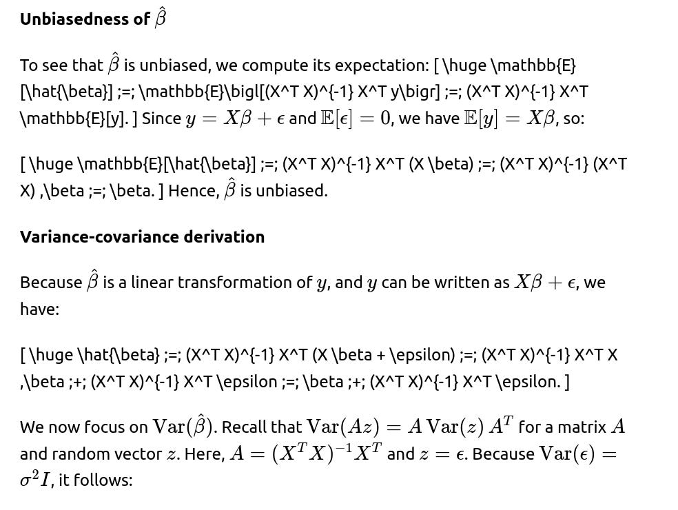
Short Compact solution

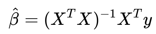
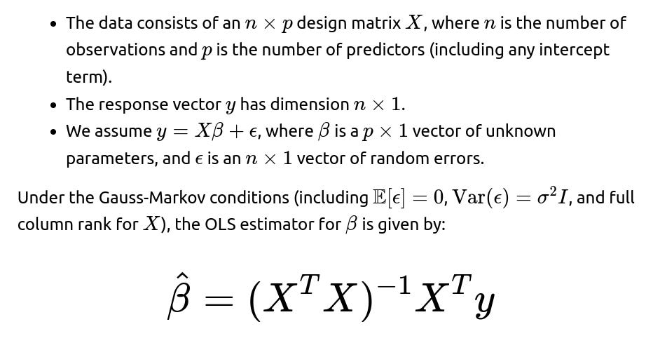
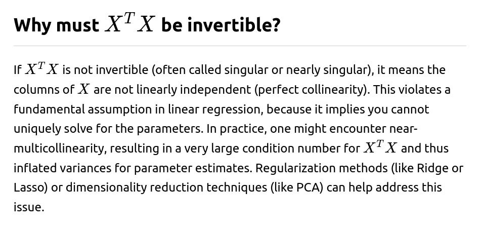
One can start with the closed-form solution for the Ordinary Least Squares (OLS) estimator:

Comprehensive Explanation

Overview and setup

We typically assume a linear regression model in the form:

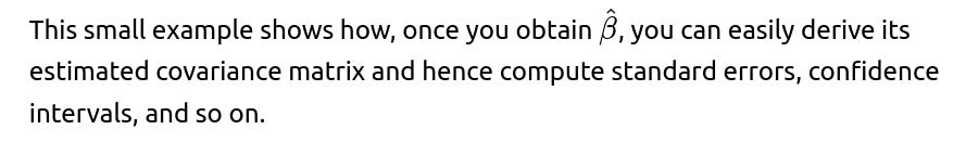
Python demonstration of computing this in practice

estimated variance-covariance matrix in Python, assuming X and y are NumPy arrays and that X already includes a column of ones for the intercept:

import numpy as np

# X is n x p, y is n x 1
# Compute OLS solution
beta_hat = np.linalg.inv(X.T @ X) @ X.T @ y

# Predicted values
y_pred = X @ beta_hat

# Residuals
residuals = y - y_pred

# Estimate sigma^2
n, p = X.shape
sigma2_hat = (residuals.T @ residuals) / (n - p)

# Variance-covariance matrix of beta_hat
cov_beta_hat = sigma2_hat * np.linalg.inv(X.T @ X)
print("Covariance matrix of estimated parameters:\n", cov_beta_hat)

Below are additional follow-up questions

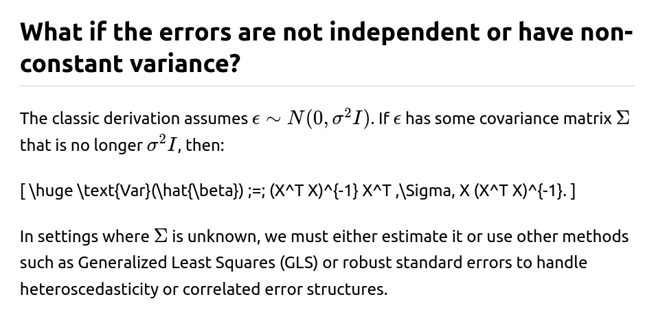
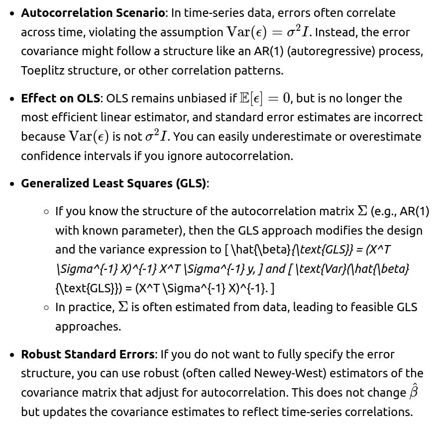
How does the distribution of ϵ affect the derivation and the resulting confidence intervals?

• Robust Methods: If the error distribution is suspected to deviate significantly, robust regression techniques (like Huber or Tukey’s biweight) can be employed, and the variance-covariance formula must be modified accordingly to reflect the robust weighting scheme.

  

  

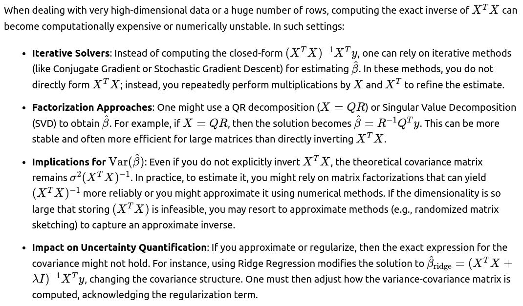
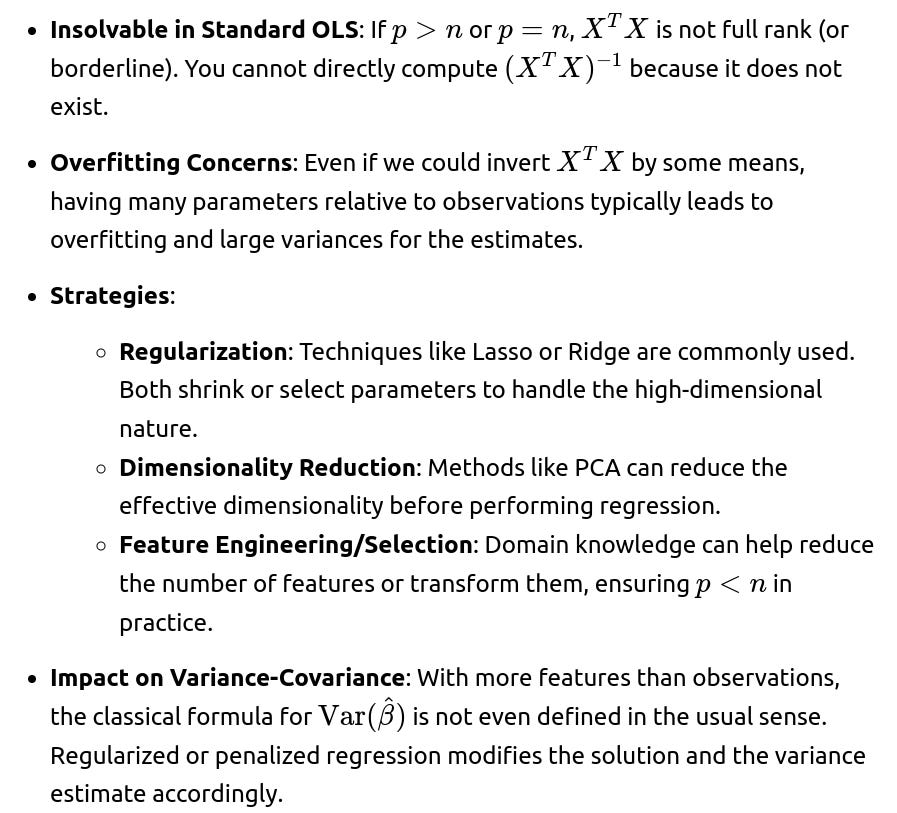
  How do we handle scenarios where p≥n (more features than observations)?

  

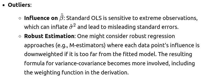
  How do we deal with the situation where some rows of X might be missing data or have outliers?

  • Missing Data:

    

    

    

    

    Can you explain how the covariance matrix changes if we use weighted least squares instead of OLS?

    

    

    

    When might you consider Bayesian approaches to estimate β and its uncertainty instead of classical frequentist OLS?

    Prior Information: If you have meaningful prior beliefs about the values of β, Bayesian methods allow you to incorporate those priors. This is especially helpful when n is small, or p is large, and you want regularized estimates that reflect domain knowledge.

  • Posterior Distribution: Instead of getting a point estimate and a covariance matrix, Bayesian methods give you a full posterior distribution for β. From this, you can compute credible intervals that may sometimes be more intuitive than frequentist confidence intervals.

  Complex Models: When the model is more complicated (e.g., hierarchical structures, correlated errors, missing data, or partial pooling across subgroups), Bayesian frameworks might offer more flexible inference and more straightforward ways to propagate uncertainty.

• Challenges:

  • Computation: Markov Chain Monte Carlo (MCMC) methods can be computationally expensive. Variational inference or integrated nested Laplace approximations (INLA) can help, but the complexity might still exceed classical OLS if the model is large or highly complex.

  • Choice of Prior: The results can be sensitive to the choice of prior if the data is not very informative. Careful domain-driven selection or robust default priors (e.g., weakly informative priors) can mitigate this.

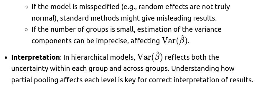
How does the variance-covariance result extend to multilevel or hierarchical models?

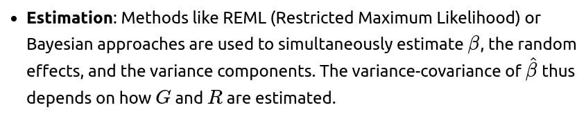
• Multilevel Model Structure: In hierarchical regression, you might have random intercepts (and possibly slopes) at group level. The model is often expressed with random effects u∼N(0,G), and residual errors ϵ∼N(0,R), where G and R capture different variance components.

  Marginal Covariance: The marginal distribution of y might be N(Xβ,V), where V incorporates both G and R. In a two-level model, V is typically block-diagonal or has a more elaborate structure depending on how the random effects manifest.

  

• Pitfalls: