
ML Interview Q Series: Simulating Standard Normal Distribution with Bernoulli Generator and Central Limit Theorem.

Browse all the Probability Interview Questions here.
Suppose you only have access to a Bernoulli generator with probability p of yielding a success. How can you draw samples that approximate a standard normal distribution from it?
Short Compact solution
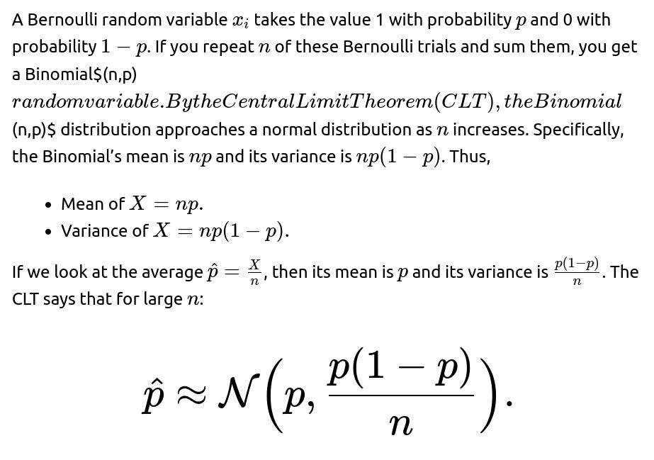
If you conduct n independent Bernoulli trials where each trial succeeds with probability p, the sum of these trials follows a Binomial$(n,p)$ distribution. Define the sample proportion as

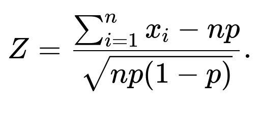
Rewriting in terms of the raw Bernoulli outcomes, we get

For sufficiently large n, Z is approximately drawn from a standard normal distribution.
Comprehensive Explanation
Why the Binomial can approximate the Normal

Use Z as an approximate draw from a standard normal distribution.
Why this Works Even with Just a Bernoulli Generator
A Bernoulli generator gives discrete outputs (0 or 1). Despite that, the sum of a large number of Bernoulli variables has a distribution that, by the CLT, “smears out” into a near-smooth bell-shaped curve. Standardizing this sum (or the sample proportion) yields a variable whose shape resembles the standard normal distribution for large n. This is effectively an application of the Binomial–Normal approximation.
Code Illustration in Python
Below is a small Python snippet that demonstrates how to generate approximate standard normal samples from a Bernoulli generator using the above approach. Suppose we have a function bernoulli_trial(p) that returns 1 with probability p and 0 otherwise.
import random
import math
import statistics

def bernoulli_trial(p):
    return 1 if random.random() < p else 0

def generate_approx_normal(p, n):
    # Sum n Bernoulli trials
    total_successes = sum(bernoulli_trial(p) for _ in range(n))
    # Standardize
    z = (total_successes - n * p) / math.sqrt(n * p * (1 - p))
    return z

# Example usage:
samples = [generate_approx_normal(p=0.3, n=1000) for _ in range(10000)]

print("Mean of generated samples:", statistics.mean(samples))
print("Std of generated samples: ", statistics.pstdev(samples))
In this example, each call to generate_approx_normal(p, n) returns one sample that is roughly distributed as a standard normal for large enough n. Over many iterations, you should see the sample mean close to 0 and the sample standard deviation near 1.
Follow-Up Question 1
How large does n need to be for the approximation to be accurate?
When dealing with binomial approximations to the normal distribution, a typical rule is that np and n(1−p) must both be at least 10 for the CLT to be reasonably accurate. In practice, if p is close to 0 or 1, you need even larger values of n to capture a decent approximation. For instance, if p=0.5, then the sum S has maximal variance, which makes the normal approximation converge somewhat faster. If p is very small or large, the distribution becomes skewed, so a bigger n is required to get a symmetric enough shape.
Follow-Up Question 2
What if p is extremely small or extremely large?
If p is near 0 or 1, the Binomial$(n,p)$ distribution becomes heavily skewed, and the normal approximation is no longer ideal for moderate n. You would need a significantly larger n to achieve a decent approximation. Alternatively, other approximations (like the Poisson approximation for very small p) may be more appropriate, though that wouldn’t necessarily yield a standard normal variable. If the only requirement is generating standard normals from a Bernoulli generator, it might be more pragmatic to implement a method to convert Bernoulli bits into a uniform distribution (e.g., using a fair-coin approach) and then apply a standard transformation such as Box-Muller. However, that requires special care to handle bias if p≠0.5.
Follow-Up Question 3
Could we construct uniform random values from a Bernoulli generator and then use a typical normal sampling method like Box-Muller?
Yes. If you have a fair coin (p=0.5), you can generate uniform values in [0,1) by treating consecutive coin tosses as bits in a binary fraction. For biased p≠0.5, you can use various algorithms (like von Neumann’s extractor) to produce unbiased coin tosses from a biased coin, though that process can be more involved. Once you can produce uniform(0,1) samples, you can apply the Box-Muller transform or other standard methods (like the Ziggurat algorithm) to produce exactly distributed standard normals rather than just approximate ones.
Follow-Up Question 4
What are the computational considerations of summing large Bernoulli trials versus using a uniform-based method?
Summing many Bernoulli trials to approximate a single normal sample might be inefficient if n is large. You would repeatedly call the Bernoulli generator n times per sample. If you need a great quantity of normal samples, this could become computationally expensive. Meanwhile, if you convert Bernoulli bits to uniform and then apply a method like the Box-Muller transform, you often generate multiple normal samples in fewer steps. The choice depends on factors like how large n must be to achieve the accuracy you want, how quickly you can convert Bernoulli outputs to uniform values, and which approach is simpler to implement for your use case.
Follow-Up Question 5
Are there any edge cases or subtle issues when using the Central Limit Theorem here?
One subtlety is that the CLT is an asymptotic statement, so it only strictly holds for large n. For moderate or small n, the approximation might not be very accurate, especially if p is near 0 or 1. Additionally, if you want to sample from a normal distribution in tails (e.g., values beyond 3 standard deviations), the Binomial-based approach may be less accurate for the extreme parts of the distribution. Practical usage typically focuses on the bulk of the distribution near the mean, where the approximation is strongest.
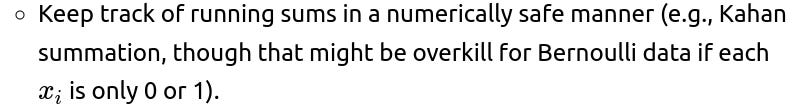
Another subtlety is ensuring your Bernoulli trials truly are independent. If there is any autocorrelation in how these Bernoulli samples are generated, you can distort the resulting distribution. Lastly, in real systems, floating-point rounding or integer overflow might appear if n is extremely large, so you have to be mindful of numerical limits.
Below are additional follow-up questions
How would we handle generating multiple correlated normal variables using only Bernoulli draws?
One might need correlated (multivariate) normal vectors rather than just independent univariate normals. Generating correlated normal variables from Bernoulli draws poses additional complexity because the naive approach—summing independent Bernoulli draws to form approximate normals—only yields independent estimates. Here are a few possible methods:
Generate each normal marginal individually, then introduce correlation: If the target correlation is relatively small or moderate, you could attempt a technique like a Cholesky decomposition on the desired covariance matrix and then feed in correlated partial sums of Bernoulli draws. In practice, you might produce an n-dimensional vector of binomial-based normal approximations, multiply it by the Cholesky factor of the correlation matrix, and then rescale so each dimension remains roughly standard normal. The challenge is ensuring you truly get the correlation you want without systematically biasing the distribution, because you are stacking many Bernoulli draws that might not be straightforward to couple across dimensions.
Use a coupling approach at the Bernoulli level: You might try to generate correlated Bernoulli variables that, when summed and standardized, yield correlated normal vectors. This can be tricky, because Bernoulli correlations do not map linearly to normal correlations. You often need custom correlation structures or specialized sampling algorithms that directly produce correlated Bernoulli sequences.
Potential pitfalls:
Maintaining the correct covariance structure is more complex than in the continuous case.
You need very large n to ensure stable approximations.
Rounding or integer overflow might appear if n gets extremely large.
In real-world scenarios, one often sidesteps this complexity by generating uniform(0,1) values first (possibly from Bernoulli bits if needed) and then applying methods for correlated normal draws (e.g., applying inverse CDF transformations or using standard multivariate normal sampling with Cholesky or PCA-based methods).
Does the speed of convergence to the normal differ based on p?
Yes, the speed of convergence under the Central Limit Theorem can vary significantly depending on p:
Near p=0.5: The binomial distribution is symmetric and has its largest variance, so the CLT typically provides a decent approximation with smaller n.
Extreme p values (close to 0 or 1): The distribution becomes skewed, and you need a larger n before the distribution’s shape is sufficiently bell-like. The tail areas, in particular, can deviate quite a bit from a perfect normal shape for moderate n.
Variance considerations: When p is very small or very large, the variance np(1−p) may be small, so the distribution can be tightly concentrated around its mean. This leads to a slower approach to the continuous normal curve, especially in the tails.
Practical impact: If p is not near 0.5, the normal approximation can misrepresent extreme outcomes. If you rely on tail probabilities for risk or anomaly detection, the approximation might be less reliable.
What happens if p changes over time in an online setting?
In real-world streaming or online scenarios, the parameter p for a Bernoulli generator might not be fixed:
Changing p: If p shifts gradually over time, the sum of Bernoulli trials might no longer come from a stationary Binomial$(n,p)$ distribution. That invalidates the straightforward application of the CLT with the same mean and variance.


Impact on normal approximation: The normal approximation still might hold locally if, over a short enough window, p doesn’t vary too much. But for large windows, the distribution becomes a mixture of binomials with different parameters, which may no longer be close to a single normal distribution.
Edge case: If p abruptly changes, you might see a “jump” in the distribution that wouldn’t be well-modeled by a single normal. One solution is to segment your data into chunks where p is relatively stable, then apply the normal approximation to each segment separately.
Are there numerical stability concerns when n is extremely large?
When n is very large, certain computations could become numerically unstable:

could be susceptible to floating-point round-off if np is large and S is on a similar scale. Subtraction of two nearly equal large numbers might reduce precision.
Mitigations:
Use a higher-precision floating type, such as double precision or arbitrary-precision libraries.
Break the computation into stable partial sums or normalized increments to avoid large intermediate values.
Does the distribution remain valid for extreme tail analysis?
A key concern in some applications, such as finance or anomaly detection, is whether the binomial-based normal approximation captures rare events in the tails:
Tail discrepancies: The normal approximation can under- or over-represent tail probabilities when n is not very large. Even if the mean region is approximated well, the CLT convergence in the tails may require substantially larger sample sizes to align with the true normal tail.
Alternative distributions: In extreme tail analyses, one might consider the Poisson approximation (when p is small) or other distributions like generalized Pareto distributions if tail events are extremely rare.
Pitfall: Overconfidence in the normal approximation can lead to underestimating the frequency of rare events (heavy tails). If your real system has heavier tails than a normal, you might systematically misprice risk or misjudge anomalies.
Could we improve the approximation with a continuity correction?
A continuity correction is sometimes used when approximating a discrete distribution with a continuous one:


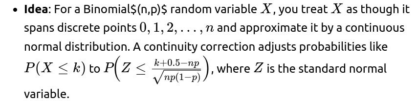
Applicability here: Since you are ultimately standardizing the sum (or mean) directly, the continuity correction might not typically be introduced in the final Z formula. However, if you’re computing exact tail probabilities or quantiles from the binomial distribution, a small shift of about 0.5 can improve alignment with the normal distribution for moderate n.
Pitfall: For large n, continuity correction matters less, but for borderline cases (like np around 10), it can yield slightly better probability estimates near integer cutoffs.
How do we interpret or handle the randomness if p itself is estimated from data?

What if we want to reuse the Bernoulli draws for multiple transformations?
Sometimes you may think: “I have a batch of Bernoulli draws. Could I generate multiple normal samples from the same set of draws?” Typically, you cannot do that if you want them to remain independent. Here’s why:
One sum per set: Once you sum n Bernoulli draws to get S for a single normal approximation, reusing those exact Bernoulli draws for another sum S′ with overlap in draws would correlate your results.
Potential approach:
If you want many independent normal samples, you need disjoint sets of n Bernoulli draws each time (or carefully designed partial overlap that still ensures independence, which is non-trivial).
If correlation is acceptable or desired, you could intentionally reuse subsets of Bernoulli draws. But that correlation might be difficult to control or quantify.
Edge case: If n is extremely large, reusing draws might not heavily degrade independence if you only overlap by a small fraction. Still, any overlap would theoretically introduce correlation.
How does the variance in the standardized variable compare if we do repeated sampling of Z?
Consider a scenario where you generate many Z values by summing fresh sets of n Bernoulli draws. Each Z is:


Expected mean: 0, if p is known exactly and the Bernoulli trials are unbiased.
Expected variance: 1, again only in the limit if n is large.
Finite-sample effect: For moderate n, the variance of Z may be slightly off from 1 due to discrete effects. It’s common to see small fluctuations below or above 1.
Pitfall: Relying on a single short run to conclude that Z definitely has variance 1 can be misleading. In real implementations, you might compute the empirical variance of Z over multiple samples to see if it’s close to 1.

Could we combine sums from smaller batch sizes to form a single normal approximation?
In some cases, you might not have the capacity to collect all n Bernoulli draws in one shot:


Pitfalls:
You must be sure that each batch is truly from the same p. If p changes over time or across batches, the combined sum is actually from a mixture distribution.
If the batch sums themselves are used in an intermediate step that modifies or biases them (e.g., weighting, normalizing differently), then the final result might deviate from Binomial$(n,p)$.
By carefully aggregating partial sums, you can still approximate a normal distribution for the final Z, but you have to ensure data consistency across batches.
How can we validate the quality of our normal approximation in practice?
Implementing checks for the approximation is crucial:
Statistical tests: You can apply normality tests (e.g., Shapiro–Wilk test, Anderson–Darling test) on the generated samples to see if they deviate significantly from a standard normal distribution.
Quantile-quantile (Q-Q) plots: Plotting the empirical quantiles of your generated Z against theoretical normal quantiles is a quick visual check. Deviations in the tails or curvature in the line can reveal problems.
Repeated sampling: Generate multiple batches of Z values and compare their sample means and variances to 0 and 1, respectively.
Pitfall: Even if the test fails at small sample sizes, it might be that n (the number of Bernoulli draws per Z) just isn’t large enough. If n is large and the test or Q-Q plot still shows consistent deviations, it might be that p is extreme, or there is bias or correlation in the Bernoulli process.
Are there alternative transformations that could improve the approximation?
Although standardizing the binomial sum is the most direct method, there are more nuanced transformations:
Wilson–Hilferty transformation: Sometimes used for chi-square distributions, but can also be extended to approximate certain discrete distributions.
Edgeworth or Cornish–Fisher expansions: These expansions can correct for skewness and kurtosis beyond the standard normal approximation. They can yield more accurate approximations for moderate n.
Practical significance: If you only need rough normal draws, such expansions might be overkill. But if your application demands high accuracy in distributional tails or mid-range probabilities for moderate n, using expansions could reduce error.
These alternative transformations involve higher-order terms in the expansion of the binomial distribution’s moment generating function and can help address the mismatch in tails or skewness that the bare-bones CLT might overlook.