ML Interview Q Series: Solving First-Head-Wins Coin Flip Game Probability Using Recursion
Browse all the Probability Interview Questions here.
Two players, A and B, alternately flip a weighted coin with probability p of landing heads. A starts first. The first head that appears determines the winner. What is the probability that A eventually wins?
Short Compact solution
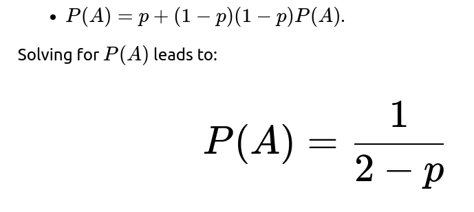
Let P(A) be the probability that A wins. If A flips a head on the first try, A wins right away. If A flips tails and then B also flips tails, the entire scenario resets to the original situation, with probability P(A) of winning from that reset point. Formally:
Comprehensive Explanation
A and B take turns flipping a biased coin that shows heads with probability p. Because A goes first, A has an inherent advantage. To see why, consider the events:
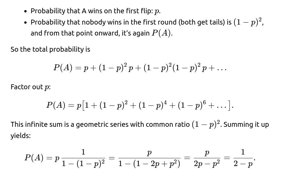
A wins on the first flip: This happens with probability p, because that is the chance of getting heads on A’s first toss.

Putting this together, P(A) is built from these scenarios. Mathematically:
A wins if the initial flip is heads.
If both A and B fail initially (both get tails), the game effectively resets.
Hence, we express it:

The key intuitive takeaway is that A retains an advantage because A always has the first chance to flip. If both fail in a cycle, it resets and A again takes the first shot in the new cycle.
Possible Follow-up Questions
Could we derive the same result using a geometric series approach?
Yes. Another way to see this is to note that, if A fails, B has a chance to win. If B also fails, we return to the original state. We can treat it as an infinite geometric series of probabilities for A winning on the first set of flips, or second set of flips (after both fail once), or the third set (after both fail twice), and so on.
We write:

How would we simulate this scenario in Python?
We could write a simple Monte Carlo simulation. For each simulation, start with A’s turn and flip a biased coin until someone gets a head. Keep track of whether A or B wins, then estimate P(A) by counting how often A wins. A minimal Python example:
import random

def simulate(num_trials=10_000_000, p=0.3):
    a_wins = 0
    for _ in range(num_trials):
        # State of the game: 0 for A's turn, 1 for B's turn
        player = 0
        while True:
            if random.random() < p:
                # Current player gets heads
                if player == 0:
                    a_wins += 1
                break
            # Switch player (0->1 or 1->0)
            player = 1 - player
    return a_wins / num_trials

prob_estimate = simulate(num_trials=1000000, p=0.3)
print("Estimated Probability that A wins:", prob_estimate)


How does this problem relate to more general Markov chain or absorbing state concepts?
We can treat this game as a Markov chain with “states” representing whose turn it is and the condition of the coin flips. The state in which one player finally flips heads is an absorbing state. The probability P(A) is the probability that the chain is absorbed in the state where A wins rather than the state where B wins. One can use standard Markov chain transition analysis to derive the same solution.
How might these ideas generalize if the coin’s bias is not constant between flips or if there are more than two players?
For three or more players, the first advantage still matters, but you would cycle through the players in order until someone flips heads. In such a scenario, each player’s probability of winning can be found by a similar method of enumerating the chance that everyone fails in each round, with added steps for the various transitions.
These expansions emphasize the power of analyzing repeated, identical (or suitably generalized) trials and leveraging geometric series, Markov chains, or states with restarts.
Below are additional follow-up questions
How many flips can we expect to happen on average before the game ends?
To determine the expected number of flips, we consider a random variable that tracks the total flips until a head appears. We first note that each “round” consists of up to two flips: one by A, then one by B (unless A already flipped heads). We can break down the analysis into smaller parts:
The probability that the game ends on A’s flip in the very first round is p. If that happens, there is exactly 1 flip.
The probability that the game ends on B’s flip in the first round is (1−p)p. If that happens, there are exactly 2 flips.


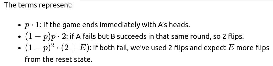

By doing this arithmetic carefully, one can find an explicit formula for E. The resulting expression will typically be a rational function of p that grows larger as p becomes small (indicating more flips are expected when heads is rare), and is smaller when p is large (fewer flips expected if heads is likely).
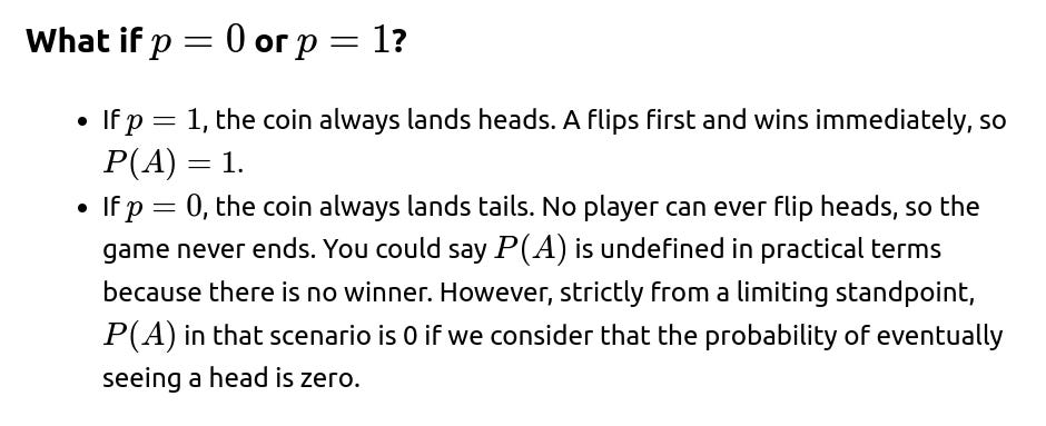
From an intuitive standpoint, when p=0.5, the expected length of the game is finite and can be computed exactly with the same technique. When p is very small (like 0.01), we expect many rounds. This underscores that p being close to 0 creates potentially long runs of tails before seeing the first head.
What if the game is limited to a fixed number of total flips?
Sometimes, the game might have a constraint such as “If no one flips a head within N total flips, the game is declared a tie.” Let’s denote that maximum number of flips by N. In that case, the analysis changes:
Each turn, you either get heads or tails. We proceed until a head appears or until we exhaust all N flips.
If no head appears by the $N$th flip, neither player wins.
To compute P(A) with a maximum of N flips, we have to consider how many flips A gets and how many flips B gets within those N flips. The number of flips each player gets depends on whether N is even or odd, and also on the order in which heads might appear.
One approach to get an exact probability in that scenario is:
Enumerate the probability of A flipping heads on flip number 1, or if the game continues, B flipping heads on flip number 2, and so on, up to the maximum N.
For each flip k, identify which player is flipping (A for odd k, B for even k).
Accumulate the probabilities that heads first appears on flip k, making sure to include the probability that all previous flips were tails.
This can be represented as:
P(A) includes the probability that the first head occurs on any odd-numbered flip (and that no head has occurred before it).
P(B) includes the probability that the first head occurs on any even-numbered flip (and no head occurred before that).
If N is large, we can also approximate by ignoring the tail scenario of no winner, especially if p isn’t too tiny. However, for smaller N or very small p, that no-winner event can be significant, and it must be accounted for properly.
How does the result generalize if we require two consecutive heads to win?
If each player needs two consecutive heads in their own turns to win, the sequence of flips gets more complicated. For instance, if A flips heads, that is not immediately a victory. On A’s next turn, if A flips another heads, A wins. But if A flips tails in between, the two-consecutive count resets. A thorough analysis has to track states such as:
“No one is on a streak.”
“A has 1 head in the streak.”
“B has 1 head in the streak.”
This is typically modeled with a finite state machine or Markov chain, because the probability of eventually reaching “A has 2 heads in a row” or “B has 2 heads in a row” can be derived from the transition probabilities among these states.
This naturally becomes more intricate than the single-head scenario, but the same fundamental approach—defining states, determining transition probabilities, and solving a system of linear equations for absorbing states—still applies. Each “streak reset” or “streak increment” leads to a different transition. Once either “A has 2 in a row” or “B has 2 in a row” is reached, that is an absorbing state.
What if there's a small probability of an erroneous flip outcome?
In some real-world contexts, one might consider an “error rate” where the coin result could be misread. For example, the coin truly lands heads with probability p, but there is a small probability ϵ that the coin reading is recorded incorrectly. Then the observed distribution of heads is not exactly p. Instead, the effective probability of seeing “heads” is p(1−ϵ)+(1−p)ϵ.
If we denote the observed (possibly mistaken) outcome’s probability of being heads by p′, then the original formula for P(A) still applies if we treat p′ as the coin’s heads probability. But the meaning of p′ is changed from the true physical bias to the “perceived” success rate. This scenario highlights that if we rely on observed flips (subject to measurement error), the advantage might shift unpredictably. Although the formula still has the same structure, the practical interpretation of p and the risk of misclassification becomes a new challenge.
What if players choose to skip their turn or pass the coin under certain conditions?
We might have a rule that a player can optionally pass their turn to the other player without flipping. That decision would be part of a strategy that might aim to maximize the probability of winning. In that case, we are no longer dealing with a simple, forced-turn game; we have a game-theoretic decision at each turn:
If you suspect that flipping at a certain time is disadvantageous, perhaps due to a certain state-based cost or a dynamic probability that changes per flip, you might skip and let the other player face a higher or lower chance of flipping heads.
To analyze such a scenario, you would invoke game theory. You would define a payoff function (1 for winning, 0 for losing, for instance) and a strategy space that includes “flip” or “skip.” Then you look for a Nash equilibrium or an optimal strategy. The straightforward 1/(2−p) formula would not directly apply anymore because the order of flipping might no longer be strictly alternating.
Could the coin flips be correlated over time?
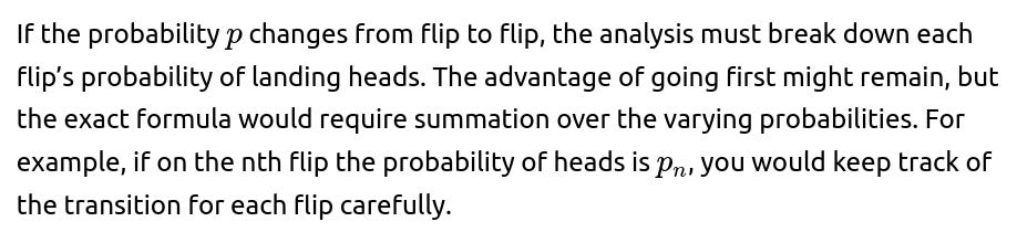
In standard treatments, each flip is independent with probability pp of heads. However, if there is correlation—maybe the coin is more likely to land heads after a previous heads, or there’s some external factor that shifts p after each flip—then the simple 1/(2−p) solution does not hold. Each new flip’s success probability and game state must be re-evaluated. In a Markov chain with correlated coin flips, you’d have additional states describing the history needed to capture correlation. The advantage of going first might still remain, but the exact probability would be derived from analyzing that larger state-space.
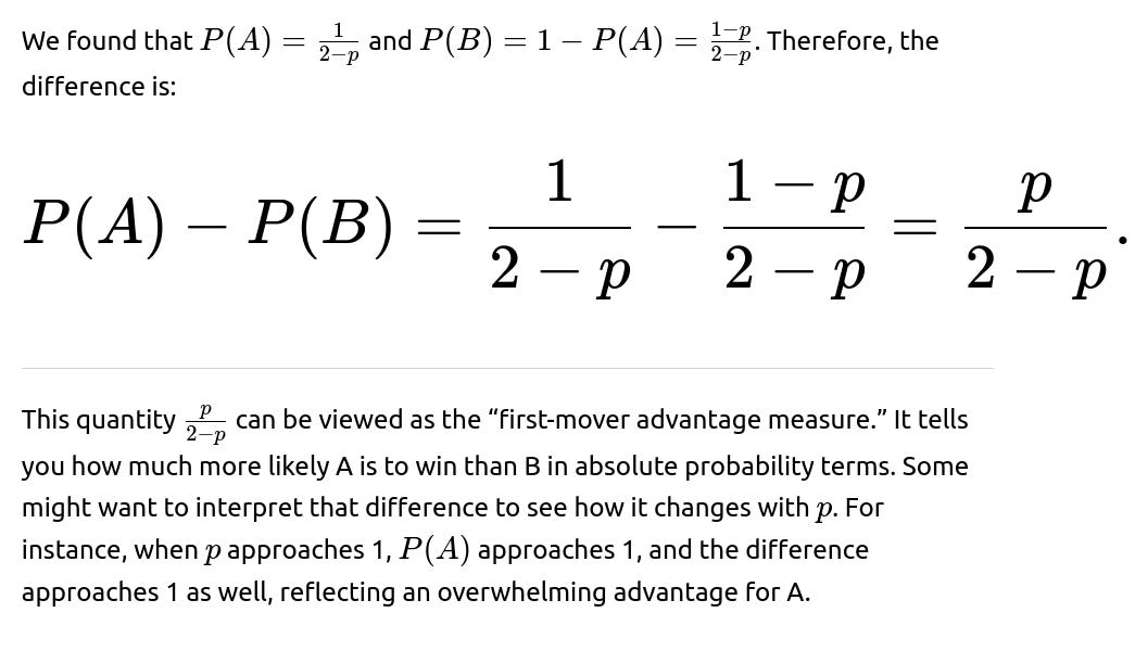
What if we are interested in the probability difference between Player A and Player B winning?

Does it matter if the coin is physically flipped at different heights or speeds by players?

Are there any real-world applications of this theoretical game setup?
One subtlety is that real-world “waiting in line” or “taking turns” processes sometimes resemble this scenario where each participant “tries” to succeed at an event with a certain success probability. For instance, in distributed systems or network protocols, multiple agents might attempt to acquire a resource or complete an operation, and the first success “wins.” While not exactly a coin flip, the same Markov or geometric approach can be applied. Pitfalls arise when:
The environment changes over time, altering success probabilities.
The resource might be locked for multiple attempts, so skipping is not allowed.
There's partial observability—participants might not fully know the outcomes of prior attempts.
In each of these real-world expansions, careful probability modeling is essential to avoid overly simplistic assumptions that might break down in practice.