
ML Interview Q Series: Solving Tennis Deuce Win Probability with Recursive Calculation

Browse all the Probability Interview Questions here.
Two contestants are in a tennis match where the score is effectively at deuce, and they keep competing until one player gains a two-point advantage. The first competitor has a 60% chance of winning any individual point, while the second competitor has a 40% chance. Determine the probability that the first competitor wins the match.
Short Compact solution
Define p as the probability that the first competitor wins the match from a neutral state. After two points are played, there are two main outcomes: the first competitor either wins both points (and thus wins immediately), or else the score returns to this same neutral state if each competitor takes one point. Mathematically:

Solving gives approximately 0.692 as the probability that the first competitor eventually wins.
Comprehensive Explanation
The problem is about a tennis situation known as “deuce,” where each competitor needs to pull ahead by two clear points to win. The first competitor has a 60% chance of winning any given point, and the second has a 40% chance. We are looking for the probability that the first competitor ultimately secures the match.
A powerful approach is to notice that after each pair of points, one of two things happens: the match either ends (because someone won two points in a row) or it resets to the original state (each competitor took exactly one point, bringing us back to the same situation as at deuce). This observation makes the problem well-suited to a Markov chain or a simple recursion because the state after a split of points effectively repeats the initial conditions.
Let p be the probability that the first competitor wins from this neutral starting point. The chance that the first competitor gets the next two points in a row is 0.6 × 0.6 = 0.36, which would immediately end the game in their favor. If the next two points are split (first competitor wins one, second competitor wins the other), the probability for that scenario is 2 × 0.6 × 0.4 = 0.48. The factor of 2 appears because there are two ways to get a 1–1 outcome in two points: (first competitor wins, second competitor wins) or (second competitor wins, first competitor wins). After such a 1–1 split, the situation is unchanged, so the probability of ultimately winning from that reset condition is again p. Hence, we arrive at
Rearranging this equation:
p − (2 × 0.6 × 0.4) p = 0.6²
p − 0.48 p = 0.36
(1 − 0.48) p = 0.36
0.52 p = 0.36
p = 0.36 / 0.52 ≈ 0.692
So, the probability that the first competitor eventually wins, starting from deuce, is approximately 0.692.
One way to interpret this is that even though the first competitor is favored (with a 60% chance per point), they still need multiple points to secure a two-point margin. The recursive structure of tennis scoring allows a relatively straightforward calculation, yielding a probability a bit under 70% that the stronger competitor wins in this scenario.
Further Follow-up Question: Why does the reset back to deuce simplify the problem?
When each competitor takes exactly one point in that two-point window, the score returns to a state that is effectively the same as the initial situation (deuce). The probabilistic nature of subsequent points is identical to the starting condition. This makes the process memoryless with respect to the state of “tied with no immediate advantage,” which is why a single probability p can describe the chance of eventually winning from that state. The game’s Markovian property (the future depends only on the present state, not on how that state was reached) is at the heart of this simplification.
Further Follow-up Question: Is there an alternative infinite series approach to solve this?
Yes, one can also view the probability of winning as an infinite geometric series. Consider all the possible patterns by which the first competitor can end up two points ahead. For instance, the first competitor could win in exactly two points, or in four points, or six points, etc., as long as the net outcome is a net of two points eventually. Each time the net advantage resets, we multiply by the factor 2 × 0.6 × 0.4 and continue. Summing those infinitely many scenarios also gives the same result after a convergent geometric series. However, the recursive equation is more concise and easier to handle computationally.
Further Follow-up Question: How do we generalize this if the probability of winning a point for the first competitor is p and for the second competitor is 1 − p?
The same approach still applies. If we let p be the probability that the first competitor wins a point, then define x as the probability that the first competitor wins the match from a neutral state. The chance of winning two consecutive points is p², and the chance of splitting points is 2 p (1 − p). Hence:

Solving for x in the same manner yields:
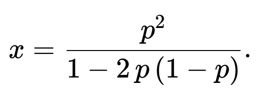
As long as p ≠ 0.5, this fraction makes sense and yields the correct probability. If p = 0.5, symmetry arguments reveal the probability is 0.5 for each competitor, which can also be derived by carefully handling the limit of that expression.
Further Follow-up Question: Can we simulate this process using Python to empirically verify the probability?
Yes, a straightforward Monte Carlo simulation will confirm our analytical result. One could run millions of simulated matches and keep track of how many times the first competitor comes out on top. An example is shown below. Keep in mind that random simulations will not yield precisely 0.692, but as the number of matches grows large, the empirical average will converge near that value.
import random

def simulate_match(prob_first_player=0.6, num_simulations=10_000_000):
    wins = 0
    for _ in range(num_simulations):
        score_diff = 0  # 0 means tied, positive means first competitor leads, negative means second leads
        while abs(score_diff) < 2:
            if random.random() < prob_first_player:
                score_diff += 1
            else:
                score_diff -= 1
        if score_diff > 0:
            wins += 1
    return wins / num_simulations

estimated_probability = simulate_match()
print(f"Estimated probability of first competitor winning: {estimated_probability}")
This script creates a large number of matches starting at deuce and uses the 60% vs. 40% odds for each point. Over many runs, you will see a result close to 0.692.
Further Follow-up Question: In real-world tennis scoring, does this logic hold if players’ probabilities of winning each point change over time?
The simple model here assumes each point is an independent trial with a fixed probability of success. In reality, players can experience fatigue or momentum swings that alter their likelihood of winning subsequent points. If the probability changes from point to point, you cannot directly apply the single recursive formula with a constant 0.6. Instead, you would need to track the evolving probability of winning each point, or create a more complex Markov chain with multiple states that capture these shifts. This can be significantly more involved but still solvable if you define enough states or use dynamic programming to incorporate changing probabilities.
Further Follow-up Question: What are common pitfalls when someone tries to solve this by enumerating possible sequences?
A typical mistake is to try listing sequences of points without noticing that infinitely many sequences can occur before someone gets a two-point lead. Failing to recognize that repeated “back to deuce” scenarios continue indefinitely can lead to an incomplete summation of probabilities. Another pitfall is neglecting the factor of 2 that arises from the different ways the points can be split in a two-point sequence. The recursive or Markov chain viewpoint is a much cleaner approach that avoids incomplete or double counting.
Below are additional follow-up questions
Could the final probability be different if we explicitly accounted for the "advantage" states in tennis scoring instead of simply returning to deuce?
In classic tennis scoring, when players are deuce, one player can gain “advantage” by winning a point, and then if they win the next point, they win the game. If they lose that next point, the score returns to deuce. This is functionally equivalent to needing a two-point lead. However, an explicit “advantage” label implies an intermediate state. For each point won by the player at advantage, the game concludes; for each point lost by the player at advantage, we move back to deuce.
Mathematically, we can represent these states:
Deuce (no one has advantage).
Advantage First Competitor.
Advantage Second Competitor.
Game concluded.
When using a Markov chain, the transitions from these states would look like:
From Deuce to Advantage First Competitor if the first competitor wins the point.
From Deuce to Advantage Second Competitor if the second competitor wins the point.
From Advantage First Competitor to Deuce if the first competitor loses the point.
From Advantage First Competitor to Game Over if the first competitor wins again.
From Advantage Second Competitor to Deuce if the second competitor loses the point.
From Advantage Second Competitor to Game Over if the second competitor wins again.
Despite enumerating these states, the final probability of the first competitor winning remains identical to the simpler two-point lead approach. The reason is that “advantage” is just a label for “one competitor is up by one.” In both methods, a two-point net lead is ultimately required, so the result is the same. The main difference is that the advantage-based approach involves more explicit states but yields the same numerical outcome.
A potential pitfall if someone tries to do it explicitly is missing the transitions back to deuce or incorrectly counting the probabilities in each step. However, once done correctly, the final answer would match the simpler recursion.
How does the probability change if the first competitor is already up by one point (or down by one point) instead of starting exactly at deuce?
If you begin from a situation where the first competitor is already ahead by one point (such as “advantage first competitor” in tennis), the probability of eventually winning is higher than from deuce. Conversely, if the competitor is behind by one point, their chance of coming back is lower than from deuce.
We can generalize the recursion for an arbitrary lead. Suppose we define:
p(i) as the probability that the first competitor eventually wins if currently ahead by i points.
The first competitor wins the match if p(i) reaches +2.
The first competitor loses if p(i) reaches −2.
We can create a system of linear equations where p(0) corresponds to deuce, p(1) corresponds to having advantage, and so on. For instance, if the first competitor has advantage (i = 1), the probability of winning the match p(1) satisfies:
With probability 0.6 (assuming the 60/40 chance), the first competitor wins the next point and thus wins the match outright.
With probability 0.4, they lose the next point and return to i = 0 (deuce). Hence, p(1) = 0.6 × 1 + 0.4 × p(0).
A symmetrical equation can handle the case when the competitor is behind by one point, i = −1. Collecting these equations yields the same final numeric value for p(0) as the simpler two-point lead recursion. A main pitfall is forgetting that p(+2) = 1 and p(−2) = 0 by definition, since those states represent finishing conditions.
If we tweak the independence assumption and allow for “streaky” behavior, how does that affect the result?
If points are no longer independent and instead come in streaks—say, if winning one point makes it more likely to win the next—then the 60% figure is not uniform. Perhaps after winning a point, the competitor’s chance for winning the next point increases to 70% for the immediate subsequent rally, or after losing a point, the chance might drop.
This scenario breaks the simple Markov property with a single state for “deuce.” Instead, we might track the outcome of the last point or even multiple prior points. One approach could be to define a Markov chain with additional states representing momentum, for instance:
Deuce with “competitor A on a streak.”
Deuce with “competitor B on a streak.”
Deuce with “no streak.”
Each streak might be self-reinforcing for a certain probability. Once momentum changes, transitions occur. These modifications make the chain more complicated. The final probability can shift significantly, and analyzing might require either a more advanced state-based dynamic program or a simulation. A major pitfall is oversimplifying the momentum effect and incorrectly reusing the standard 60% recursion, which would produce an inaccurate result under streaky conditions.
Could there be an edge case if p = 1 or p = 0, or if p is extremely close to those limits?
When p = 1, meaning the first competitor always wins every point, the probability of winning the match from deuce is clearly 1. Conversely, when p = 0, meaning the first competitor always loses every point, that competitor has zero probability of winning the match.
A more subtle boundary case is if p is extremely close to 0 or 1. In such scenarios, the recursion is still valid, but numerically, if p is near 0.9999, even though you might expect almost certain victory, you still need to be mindful of the floating-point arithmetic in a simulation. In actual code, a large number of iterations might be needed to verify the probability accurately. A big pitfall is that standard double-precision floating-point might start to give rounding errors if p is extremely close to 1 or 0. In symbolic or high-precision arithmetic, it would be unambiguous that p = 1 leads to a 100% chance and p = 0 leads to a 0% chance.
How does the concept generalize to a “win by k points” scenario instead of “win by 2” from a tie state?
In some variants of sports or games, you must pull ahead by k points. We can label the probability that the first competitor wins (starting from a tie 0–0) as P. In each round, the first competitor’s chance of winning one point is p, and the second competitor’s is 1 − p. You can track states by how many points each competitor is ahead or behind. For a “win by k” system, the boundary states become +k (first competitor wins) or −k (second competitor wins).
One direct extension is:
Let P(i) be the probability that the first competitor eventually wins if they are i points ahead.
When i = k, P(k) = 1, and when i = −k, P(−k) = 0.
For −k < i < k, we have:
P(i) = p × P(i+1) + (1 − p) × P(i−1).
Solving these difference equations yields the probability from i = 0. A potential mistake is incorrectly skipping states or inadvertently reverting to the “win by 2” formula, leading to an incorrect final probability. The number of equations grows, but the logic is the same: you look for the net lead to reach k or −k.
What happens if we attempt to approximate the probability with a “continuous” view (like a random walk or Brownian motion analogy)?
Sometimes people try to approximate a discrete random walk with a continuous diffusion process to gain intuition for large k or large numbers of points. If each point is a Bernoulli trial with probability p, then the difference in score is a random walk. In principle, for a large “win by k” scenario, this random walk approach can be approximated by a Brownian motion with drift (where the drift is p − (1 − p) = 2p − 1). The probability of eventually hitting +k before −k in a continuous model is well known in stochastic processes.
However, for the small k = 2 scenario (typical tennis deuce), a continuous approximation does not add much clarity. It’s more relevant for large “win by difference” settings. A subtle pitfall is that a continuous approximation can break down for small k, leading to an unintentional introduction of error. In short, discrete methods are simpler and exact for small k.
How should we interpret or adjust for real-life tennis factors like serving rotation, second serves, or tie-breaks?
Real tennis does not strictly have a 60% or 40% chance on every single point, because certain points are served by one player, others by the opponent. Additionally, second serves might carry different probabilities of success. In actual tennis, we can break it down:
Determine who is serving at each point in the deuce scenario.
Adjust the probability that the server wins a point, which might be different from the probability that the receiver wins.
If the first competitor is the server in deuce, they might have a 60% chance of winning that service point. After that point, either they continue to serve (in some formats) or it might switch in other variants. Another dimension is double faults or aces that skew the distribution further. If these aspects are relevant, the standard “each point is independent with the same 60% chance” model fails. You’d either compute a more comprehensive Markov chain, tracking who serves each point, or run a simulation with the appropriate serving probabilities. A typical pitfall is incorrectly assuming you can just apply a single uniform probability per point throughout the entire deuce sequence if the serve is switching in a structured pattern.
In coding simulations for this scenario, what are some numerical pitfalls or edge cases?
Randomness Quality: If someone uses a pseudo-random generator improperly or seeds the generator in a loop incorrectly, results can be biased.
Insufficient Iterations: To reduce random noise, you need a sufficient number of iterations. With too few, the empirical probability might deviate significantly from the true value.
Edge Cases (p = 0 or 1): If p is set to 0 or 1, the code might have a loop that runs infinitely or never enters certain conditions. Proper checks or break conditions are needed.
Floating-Point Summation: If you implement a summation-based approach (like an infinite series for repeated returns to deuce), extremely small terms may cause floating-point underflow, or large partial sums may cause floating-point overflow.
Guarding against these pitfalls involves thorough testing, including edge cases, and confirming the simulation results with known exact values for simpler scenarios (like p=0.5 or p=1) where we already know the outcome.
Is there a closed-form expression for this probability when p ≠ 0.5, and how might we derive it using infinite series?
Yes, we can derive a closed-form expression using infinite series. One way is:
Probability that the first competitor wins in exactly 2 points: p².
Probability that it returns to deuce: 2 p (1 − p). After returning to deuce, the probability of eventually winning remains the same, so we multiply by p again.
Hence, summing over infinitely many returns to deuce:
p = p² + [2 p (1 − p)] p + [2 p (1 − p)]² p + [2 p (1 − p)]³ p + …
Factor out p²:
p = p² [1 + 2 p (1 − p) + (2 p (1 − p))² + (2 p (1 − p))³ + … ]
This is a geometric series. The sum of an infinite geometric series 1 + r + r² + … is 1 / (1 − r) for |r| < 1. Here, r = 2 p (1 − p). Hence,
p = p² / [1 − 2 p (1 − p)] = p² / [1 − 2p + 2p²].
Simplifying, p = p² / [ (1 − p)² + p² ]. If p = 0.6, plugging in yields approximately 0.692. The main pitfall is forgetting to factor out the correct terms or incorrectly summing only a finite number of terms in the infinite geometric series. To avoid that, always verify the ratio 2 p (1 − p) is strictly less than 1 (which it is for 0 < p < 1), ensuring convergence.
Can we interpret this recursive approach in relation to gambler’s ruin problems?
This scenario is indeed structurally akin to a gambler’s ruin problem, where the difference in points is the gambler’s capital, and “ruin” happens when the capital hits −2 relative to some baseline, while “success” happens at +2. The difference is that here we re-center at 0 each time we get back to a tie, but the underlying mechanism—a Markov chain with absorbing boundaries—is the same. For gambler’s ruin, states are the integer amounts of wealth. For tennis deuce, states are point-differences between players. One subtlety is that “return to zero” can happen repeatedly, just like returning to some intermediate capital in gambler’s ruin. The pitfall is not recognizing that tennis scoring is just a special case of an absorbing Markov chain with states from −∞ to +∞, truncated in practical terms once we get ±2 from the baseline.
Is it possible for a very large advantage to “collapse” back to deuce in a real match?
In a single game of tennis, you never literally become more than one point up after deuce, because as soon as you’re one point up at deuce, that’s called “advantage.” If you win another point, you win the game and do not go to a +2 lead beyond that moment. The two-point difference is checked immediately upon each point. So you effectively get a maximum lead of +1 at the deuce stage before the game ends at +2. Collapsing from +1 (advantage) back to 0 (deuce) can and does happen. However, you cannot be, for instance, +3 after deuce, as the game would have ended at +2. A practical pitfall is mixing up game-level scoring with set-level or match-level scoring, which can involve multiple games and can indeed produce bigger swings in leads and deficits.