
ML Interview Q Series: Statistical Hypothesis Testing to Detect Bias in Coin Flips
Browse all the Probability Interview Questions here.
How can you determine if a given two-sided coin, which might be fair or biased, is actually biased, and how would you identify that bias based on the test outcome?
Comprehensive Explanation
A common statistical approach to determine if a coin is biased is to perform a hypothesis test. Consider a classical hypothesis testing setup:
Null Hypothesis (H0): The coin is fair, meaning its probability of landing heads is 0.5. Alternative Hypothesis (H1): The coin is biased, meaning the probability of landing heads differs from 0.5 (it could be greater or less).
One way to test this hypothesis is to flip the coin n times and count how many times it lands heads (let’s denote that number by k). If the coin is truly fair, the number of heads follows a binomial distribution with parameters n and p = 0.5. Formally, for k heads out of n flips:
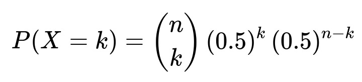
Where X is the random variable representing the number of heads. Here, n is the total number of flips, and k is the observed count of heads.
Once you have the observed k, you compute the probability of observing an outcome that is at least as extreme (either too many heads or too few heads) as what you got under the assumption that p = 0.5. This probability is the p-value. If it is less than a chosen significance level (for example, 0.05), then you reject the null hypothesis in favor of concluding that the coin is likely biased.
If the p-value is greater than the significance level, you fail to reject the null hypothesis and have insufficient evidence to state that the coin is biased (though it does not guarantee fairness; it simply fails to provide enough evidence against it).
A practical test might look like this in a step-by-step manner:
Flip the coin n times. Count the total number of heads k. Calculate the probability (p-value) of observing k or more extreme results (either far too many heads or far too few) assuming p = 0.5. If that probability is below the threshold (for instance, 0.05), conclude that the data suggests the coin is biased. If not, conclude that the data does not provide enough evidence to declare the coin biased.
The outcome that strongly indicates bias is one that yields a small p-value, meaning the observed distribution of heads is unlikely to come from a fair coin.
It is often helpful to decide on the number of flips before conducting the test, to ensure the test has enough statistical power. An insufficient number of flips might fail to detect a genuine bias (Type II error), whereas a very large number of flips might detect even slight deviations from p = 0.5.
How many flips should be performed to detect bias effectively?
The number of flips depends on the desired confidence level and the magnitude of the bias one wants to detect. Generally, if the bias is severe (for instance, the coin lands heads 80% of the time), fewer flips are needed to expose that bias. If the deviation from 50% is slight (for example, 52% heads instead of 50%), more flips will be required to confirm that difference at a certain statistical power. Practitioners often use standard sample size formulas or power analysis to decide how many flips are required to detect a specified effect size with a certain probability of success.
Can a Bayesian approach be used instead?
Yes, a Bayesian approach can certainly be adopted, where one starts with a prior belief about the probability of heads. After flipping the coin a certain number of times and observing the outcomes, one updates the prior distribution to a posterior distribution over p. A posterior heavily skewed away from 0.5 suggests strong evidence that the coin is biased. This approach can also incorporate prior knowledge or beliefs about how likely it is that the coin is fair versus biased in a certain way.
What about Type I and Type II errors?
Type I error is rejecting the null hypothesis (the coin is fair) when in fact the coin is fair. Setting the significance level (for instance, 0.05) controls the probability of this error. Type II error is failing to reject the null hypothesis (that the coin is fair) when the coin is actually biased. This depends on the test’s power, which is the probability that the test will detect a certain degree of bias if it truly exists. Increasing the number of flips increases the power, which reduces the chance of a Type II error.
Could real-world conditions affect the result?
Real-world factors such as flipping technique (force of the flip, angle of release) can introduce subtle biases. Therefore, consistent flipping and a large enough number of trials help mitigate random anomalies. Additionally, if the coin is physically imbalanced in some way, the probability of heads could deviate from 0.5 even under a standard flipping technique. If we needed to separate flipping technique from the coin’s inherent bias, we could introduce randomization in how the coin is tossed or examine different tossing methods.
What if the coin can land on its edge?
In theory, a coin can land on its edge, though the probability is typically quite small. If that outcome becomes non-negligible, the analysis requires adjusting for the third outcome. Instead of a simple binomial distribution with p for heads and 1 – p for tails, you might have probabilities p heads, q tails, and r for the edge, with p + q + r = 1. Testing for fairness then becomes more involved, but the principle remains the same: gather enough data to estimate these probabilities accurately and determine whether p or q differs significantly from 0.5 (and if r is non-negligible).
Ultimately, whether the coin is biased is determined by statistically significant deviation from p = 0.5, and the key factor is how extreme the observed frequency of heads is, given a sufficiently large number of flips.
Below are additional follow-up questions
Could a confidence interval approach be used to determine if the coin is biased, and how does that differ from hypothesis testing?
A confidence interval provides an estimated range for p (the probability of heads). For instance, if we flip the coin n times and observe k heads, we can construct an interval [L, U] that contains the true p with a certain confidence level (often 95%).
If 0.5 is not in [L, U], this suggests the coin is biased because the range in which p likely resides excludes 0.5. Conversely, if 0.5 is within the interval, we do not have enough evidence to claim a bias.
One difference from the standard hypothesis testing approach is that confidence intervals show a range of plausible values rather than a single p-value for deciding whether to accept or reject a hypothesis. This can give a more direct sense of how large or small the bias might be. However, confidence intervals and hypothesis tests are closely related concepts (for a given confidence level and significance level, they typically yield consistent conclusions regarding bias).
Potential pitfalls:
Misinterpretation of confidence intervals is common. A 95% confidence interval does not mean there is a 95% probability that p lies in that range; rather, it means that if we repeated the experiment many times, about 95% of those intervals would contain the true value of p.
Small sample sizes can yield very wide intervals, leading to inconclusive results.
What if the coin’s bias changes over time?
In real scenarios, the probability of heads could shift due to wear on the coin, differences in the flipping technique as time goes on, or subtle environmental changes (such as humidity affecting the coin’s surface). A standard hypothesis test assumes a consistent p across all flips.
When p might change over time, we have to adopt methods that account for time-varying probability. One possibility is a sliding window approach where we test smaller sets of flips in sequence to see if the estimate of p changes. Another is a Bayesian updating model that continuously refines the distribution of p and checks for drifts.
Pitfalls:
Using standard binomial assumptions across changing conditions can mask an actual variation in bias.
Over-segmentation (testing too many small windows) can increase Type I errors because repeated testing inflates false positives if not adjusted properly.
How can we make our test cost-effective if we have limited resources for coin flips?
When flips are expensive or time-consuming, we might consider statistical techniques that extract information more efficiently. One approach is to use a sequential test (like the Sequential Probability Ratio Test) that lets us stop early if data strongly indicates bias or fairness.
Pitfalls:
Stopping too early might mean missing subtle biases because the test lacks sufficient data for smaller deviations from p = 0.5.
A carefully designed stopping rule is necessary to maintain a known false-positive rate.
What if we only have partial data or missing observations from some flips?
In some scenarios, you may lose track of certain flips, or the outcome might not be properly recorded. Dealing with missing data can introduce biases if not handled correctly.
Strategies to handle missing data include:
Imputation methods (e.g., imputing an expected value based on previously observed frequencies).
Analysis restricted only to the complete data, though this might reduce your effective sample size.
Pitfalls:
Wrongly imputing missing outcomes can distort the final conclusion if the missing mechanism is not random (for example, if tails results are more likely to be unrecorded).
If the amount of missing data is significant, neither hypothesis testing nor interval estimation might yield a reliable conclusion.
Could we adopt a randomization test or a resampling-based approach if we do not want to rely on exact binomial assumptions?
A randomization (or permutation) test can compare the observed distribution of heads and tails to distributions generated by hypothetical fair-coin sequences. By permuting or simulating fair-coin outcomes many times and comparing them to the real data, one can compute a p-value that reflects how often simulated fair-coin results look as extreme as the real data.
Pitfalls:
If the coin flips are not independent or have some underlying structure (e.g., the flip technique changes over time), randomization tests may not fully capture that dependency.
Computational expense can be high for large n when repeated simulations are needed.
How can we ensure independence of flips, and why does it matter?
Independence means each flip’s outcome has no bearing on the next. If flips are not independent (for instance, if the way you flip depends on whether the last flip was heads or tails), standard binomial tests no longer hold.
To ensure independence, the flipping process must be consistent: same force, minimal knowledge of prior results while flipping, and no feedback loops that adjust the technique. For rigorous experiments, machine-based flipping mechanisms or carefully controlled hand flips are used.
Pitfalls:
If each flip’s outcome influences the next, the outcomes might follow a Markov chain rather than a simple binomial process. This invalidates many standard statistical tests unless they are adapted for dependent data.
Overlooking small correlations can lead to incorrect significance levels or confidence intervals.
How can we estimate the magnitude of the bias if the coin proves biased?
Once it appears the coin is not fair, you might want to know how different from 0.5 it is (say 0.52, 0.60, etc.). The simplest unbiased estimator of p is k/n (the number of heads divided by total flips). Maximum likelihood estimation from the binomial distribution also yields this ratio, k/n, as the MLE for p. You can refine this by constructing confidence intervals around p, or by adopting Bayesian methods with a Beta prior for more nuanced estimates.
Pitfalls:
With small n, the estimate of k/n can vary widely from the true p. Low sample sizes lead to higher uncertainty.
If there is a cost to each flip, you might decide to stop as soon as you detect the coin is biased enough for your practical use case, but that could cause wide confidence intervals around the exact bias estimate.
Could data collection or measurement errors affect the conclusion?
If the way flips are recorded is prone to human error (e.g., accidentally recording a tail when it was actually a head), the data itself can become biased. This is known as measurement error or misclassification error.
Remedies include:
Using automated or carefully double-checked methods of recording outcomes.
Performing a pilot test to estimate the rate of recording mistakes and correcting for that if possible.
Pitfalls:
Even a small error rate can obscure small biases in the coin or create an artificial bias in the results.
If errors are non-random (for instance, if one observer tends to record heads more accurately than tails), the test results can systematically shift away from reality.