
ML Interview Q Series: Steady-State Vehicle Replacement Rate: Modeling Failure Probability and Finite Lifespan.

Browse all the Probability Interview Questions here.
10. Suppose there is a new vehicle launch upcoming. Initial data suggests that on any given day there is a probability p of either a malfunction or a crash, requiring replacement. Additionally, each vehicle that has been around for n days must be replaced. What is the long-term frequency of vehicle replacements?
One way to think about this is to imagine a large population of vehicles in steady state. Each vehicle can survive at most n days because on the nth day, it must be replaced (even if it never malfunctioned or crashed before). On any day before that forced replacement, there is a probability p that a vehicle fails and needs to be replaced immediately.
The key insight is that the same fraction of vehicles that leave each day must be replaced by new ones (to keep the overall population size stable). We denote the fraction of vehicles that are newly introduced (and thus also the fraction that is removed) on a given day in the long-term equilibrium as
Below is a step-by-step intuitive explanation (without revealing hidden chain-of-thought but still providing a clear, in-depth reasoning):
You can label each vehicle by its “age in days” from 0 up to n-1. Because any vehicle is forced out on the nth day, no one can live beyond age n-1. Denote by ( x_k ) the steady-state fraction of vehicles of age k on any given day. You have:
( x_0 ) is the fraction of brand-new vehicles introduced that day.
For 0 ≤ k < n-1, ( x_{k+1} ) is the fraction of vehicles that survive from age k to age k+1. Survival means they did not fail (probability ( 1 - p )) on that day. Hence ( x_{k+1} = x_k ,(1 - p) ).
The fraction for each k must sum to 1, i.e. ( \sum_{k=0}^{n-1} x_k = 1 ).
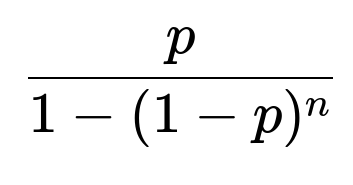
From the geometric-like progression, you obtain ( x_k = x_0 ,(1 - p)^k ). Summing from k=0 to k=n-1,

Because ( x_0 ) is precisely the fraction of vehicles replaced by new ones each day (in a steady population, each day’s newcomers exactly match each day’s departures), the fraction of daily replacements is
This fraction accounts for both the probability p of failing at any age plus the forced replacement once a vehicle reaches age n days.
You can confirm this formula by testing edge cases:
If ( p \to 0 ) (no malfunctions or crashes), then replacements only happen after n days. In that scenario, the fraction of replacements each day approaches ( \frac{1}{n} ). Indeed, as ( p \to 0 ), the expression becomes ( \frac{0}{1 - (1)^n} ) in limit form, but a proper series expansion confirms it goes to ( 1/n ).
If ( p = 1 ) (vehicles always fail immediately), everything is replaced daily, matching the fraction 1. Plugging p=1 into the expression gives 1 as well.
Below are a few potential follow-up questions that a knowledgeable interviewer might ask to test deeper understanding, and their detailed answers:
How do you handle the situation if p is extremely small but non-zero?
When ( p ) is extremely small but not zero, most vehicles will survive until the forced replacement at day n, but a small fraction will fail in between. Mathematically, ( (1 - p) \approx 1 ), so you can expand ( (1 - p)^n \approx 1 - np ) (using a first-order approximation for small ( p )). In that scenario,

Hence in practice, when ( p ) is very small, the fraction of replacements per day is very close to ( 1/n ) because most replacements come from the forced replacement after day n.
A subtlety arises if you want to track extremely rare failures over a long time: you might need a large enough fleet or long enough observation period to see those rare malfunctions. In industrial practice, you might gather data over many days (or many vehicles) to estimate p precisely.
What if we wanted to simulate this replacement process in code to empirically estimate the long-term fraction?
You can run a Monte Carlo simulation in Python. For a sufficiently large population, keep track of the age of each vehicle, randomly replace those that fail on a given day with probability p, and also replace any vehicle that reaches day n. After many days, you estimate the fraction of vehicles replaced per day. A simple prototype might look like:
import numpy as np

def simulate_replacements(num_vehicles=10_000, n=5, p=0.02, num_days=10_000):
    # Initialize all vehicles with random ages 0..n-1 to approach approximate equilibrium quickly
    ages = np.random.randint(0, n, size=num_vehicles)

    total_replaced = 0

    for day in range(num_days):
        # Probability p of failing
        failures = np.random.rand(num_vehicles) < p

        # Forced replacements (age == n-1)
        forced = (ages == (n - 1))

        replaced = failures | forced

        # Count how many replacements happened
        replaced_count = np.sum(replaced)
        total_replaced += replaced_count

        # Replace with new vehicles (age=0)
        ages[replaced] = 0

        # Increment age for vehicles that were not replaced
        ages[~replaced] += 1

    avg_replaced_per_day = total_replaced / num_days
    fraction_replaced = avg_replaced_per_day / num_vehicles
    return fraction_replaced

# Example usage
if __name__ == "__main__":
    est_fraction = simulate_replacements(num_vehicles=10000, n=5, p=0.02, num_days=20000)
    print("Estimated fraction of daily replacements:", est_fraction)
Over a large number of days, est_fraction should be close to the theoretical value
theoretical_fraction = 0.02 / (1 - (1 - 0.02)**5)
print("Theoretical fraction:", theoretical_fraction)
This kind of simulation is helpful if the process is more complicated in practice (e.g., time-varying p, multiple forced replacement rules, etc.).
How does this logic extend if there are additional complexities, such as partial repairs instead of complete replacements or multiple distinct malfunction probabilities?
You can adapt the same reasoning if the forced replacement day is still n but the malfunction probability p varies with age or with other factors. The difference would be that each age might have a different probability of malfunction, say ( p_k ) at age k. Then you’d track the steady-state fractions age by age with the updated transitions:
Probability ( 1 - p_k ) of surviving from age k to k+1.
Probability ( p_k ) of failing (leading to replacement) at age k.
A forced replacement still occurs at age n. You would sum up the probabilities of failing at each age plus the forced replacements at the last age. The final fraction introduced each day ( x_0 ) must again satisfy a consistency equation ensuring that the total fraction of vehicles across all ages is 1.
For partial repairs (where you might not replace the entire vehicle but partially fix it so it effectively “resets” the age or changes the failure probability), the Markov chain becomes more intricate: you’d have transitions to different states (maybe a state representing “repaired age 0” or “repaired age k,” etc.). The basic principle—finding a stable distribution in a Markov chain—still applies, but you set up a transition matrix for all relevant states and solve for the steady-state distribution. From there, you can calculate the fraction of replacements (or repairs) per day in the long run.
What if vehicles are replaced in batches rather than on a vehicle-by-vehicle basis?
Even if replacements occur in batches, you can still look at the entire population fractionally. The logic doesn’t change because we’re essentially analyzing the probability that any given vehicle leaves the pool in a day. Whether they leave individually or in groups doesn’t affect the total fraction that departs daily in the long-run equilibrium. As long as each individual vehicle has the same forced out date n and daily malfunction probability p, you get the same average departure fraction. Practically, you might see “surges” in replacement in real time (batch replacements of entire fleets at once), but averaged over a long enough period, the fraction remains the same.
How to confirm there is no double counting of failures and forced replacements for the vehicles that are on their nth day?
A common confusion arises around vehicles that are on day n-1 (meaning they will be replaced at the end of the day no matter what). If one of those vehicles fails earlier in that same day, it might seem we are double counting. However, in the steady-state fraction analysis:
“Malfunction replacements” from the entire population on day d is the probability p times the fraction of vehicles of all ages (which is 1 in total).
Among those at age n-1, some subset is failing that day (counted in that p fraction). Meanwhile, the rest of the age n-1 vehicles that did not fail are still forced out at the end of that day. So effectively, 100% of the vehicles at age n-1 are gone by day’s end.
In the daily fraction formula, we combine “failures at any age” plus “forced replacements at age n-1 (for those that did not fail).” The end result matches the fraction ( x_0 ) in steady state, which simplifies exactly to

Hence there is no net double counting: the fraction that fails at age n-1 is included in the p portion, and the fraction at age n-1 that does not fail is accounted for in the forced replacement portion. Summing them yields ( x_0 ), the total fraction leaving.
How might this result apply to a real-world scenario like Tesla’s vehicle monitoring?
In a real production environment, Tesla might have an entire fleet of test vehicles for a new model, each continuously monitored. Every day:
A fraction p of vehicles might have a critical failure that forces an immediate replacement.
Any vehicles that reach n days of continuous usage (without a forced replacement earlier) get replaced automatically on the nth day.
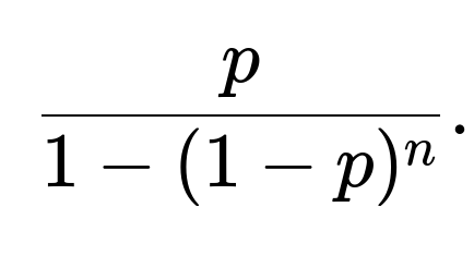
They want to know: In the long run, what fraction of the fleet is replaced each day on average? This fraction can be used for planning maintenance staff, spare parts availability, manufacturing schedules, and so forth. The formula
gives a direct, stable, long-term daily rate of replacements (as a fraction of the total fleet). It helps in resource allocation and scheduling. If Tesla modifies p (improving reliability) or extends the forced replacement day n, the fraction changes accordingly, letting them compute how the daily replacement load evolves.
In practice, if p is itself a function of time or usage conditions, or if n is not always fixed (some vehicles might be allowed to run longer if they pass certain tests), the basic idea remains the same, though the computations can become more involved.
How do we handle a scenario where vehicles do not get replaced exactly on the nth day but instead have a probability q of forced replacement on day n?
If the rule changes to “on day n, the vehicle is replaced with probability q, and otherwise continues,” you add that partial forced replacement probability into the chain. The transition from age n-1 to age n would then have a probability 1-q of continuing. You would need to set up the corresponding Markov chain with states 0 to possibly infinite, because if q<1, a fraction might survive beyond age n. However, if there is eventually some maximum day m where you absolutely must replace the vehicle, then the chain is finite, and the same approach (but with more complicated transitions) yields a closed-form or numeric solution for the steady-state distribution. The essence is always:
Define a transition probability matrix among the possible age states.
Solve for the steady-state distribution of that Markov chain.
Calculate the fraction that leaves in a single day from that steady-state.
Below are additional follow-up questions
What if the replacement day n is itself random, governed by some probability distribution rather than a fixed integer?
In many real-world scenarios, the forced replacement schedule might not be uniformly applied on a fixed day n. Instead, there could be a probability distribution specifying that each vehicle is replaced at different times. For instance, you might have a distribution where 80% of vehicles get replaced around day n, but the rest get replaced closer to day n+1 or n+2, subject to resource constraints or scheduling factors.
In that case, you no longer have a strict “maximum age.” Instead, each vehicle’s age at replacement is governed by two factors:
The chance p of failing on any given day.
A random “scheduled replacement day” ( N ), drawn from a discrete or continuous distribution.
To handle this scenario, you can model the process using a Markov chain with (theoretically) infinitely many states, each representing the vehicle’s age in days. The probability a vehicle transitions from age k to k+1 is ( 1 - p ) times the probability that it is not replaced by scheduling on that day. If the distribution is discrete, you add an extra probability that the vehicle is replaced at age k according to the scheduling distribution. Formally, you define:
( r_k ) = Probability that the vehicle is forced out (scheduled) exactly at age k, not earlier.
On any given day for age k, the probability of continuing to age k+1 is ( (1 - p)(1 - r_k) ).
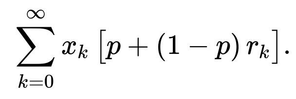
The probability of leaving on that day (via failure or scheduled replacement) is ( p + (1 - p),r_k ).
With this more complex transition mechanism, you calculate the steady-state distribution by solving for the stationary probabilities ( x_k ). Then, the long-term fraction of daily replacements is the sum of (stationary probability of being in each age k) (\times) (probability of leaving at age k). In mathematical terms, if the fraction of vehicles at age k in steady state is ( x_k ), the daily fraction replaced is:
A typical pitfall is incorrectly summing these probabilities if there’s overlap between random replacement scheduling and malfunctions on the same day. You need to ensure you account for the fact that even on a scheduled replacement day, a fraction of vehicles may have already failed earlier that same day. In an actual implementation, you must precisely define the order of events (does scheduling occur at the start of the day or end of the day? Do vehicles that fail in the morning still count for forced replacement at night?). These details matter for an accurate calculation.
Another subtlety is the data collection in real life: you need to track how many replacements occurred due to scheduling vs. how many due to malfunctions, to estimate p and the distribution of forced replacement ages. If you only know the final replacement times without distinguishing the cause, you can conflate forced replacements with failures.
How does the analysis change if p itself is time-dependent, increasing or decreasing with vehicle age?
In real-world usage, the likelihood of failure might change over time. For instance, early “infant mortality” failures might be higher just after launch (p is larger at low age), while a stable middle period might have low p, and then late “wear-out” failures might see p increase again. One way to capture this is:
Let ( p_k ) be the probability that a vehicle of age k malfunctions on a given day.
Now your Markov chain transitions are:
From age k to k+1 with probability ( 1 - p_k ), assuming no forced replacement yet.
Or immediate replacement if forced or if a malfunction happens.
With a fixed forced replacement at day n, no vehicle can get older than n-1. You then have states k = 0, 1, 2, ..., n-1, and a forced transition at k = n-1. The difference is that each transition from k to k+1 uses ( 1 - p_k ) instead of ( 1 - p ). To find the stationary distribution, you must solve:
( x_1 = x_0 (1 - p_0) )
( x_2 = x_1 (1 - p_1) )
( \dots )
( x_{n-1} = x_{n-2} (1 - p_{n-2}) )
And you still have:

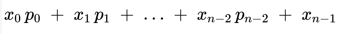
Solving iteratively,

Then impose the sum-to-one condition to solve for ( x_0 ). Once you have ( x_0 ), you can compute the fraction replaced each day (in the long run) by summing the fraction that leaves each age state:
Vehicles of age k fail with probability ( p_k ).
Vehicles of age k = n-1 get forced out if they don’t fail earlier that day.
Hence the daily fraction replaced is:
since all vehicles at age n-1 will be replaced that day, either by failing or by forced replacement.
Pitfalls here include:
Handling the possibility that p might be zero at some ages, or extremely high at others.
Data sufficiency for estimating each ( p_k ) if you have limited historical data. You’d need enough vehicles at each age to get a reliable estimate.
Implementation complexity: you must be sure you track the age distribution carefully if you attempt an empirical or simulation-based approach.
Could correlated failures between vehicles affect the steady-state fraction of replacements?
Yes, if one vehicle’s failure on a given day increases (or decreases) the likelihood of failure for other vehicles, the assumption of independence (each with probability p) no longer holds. This might happen if there is a shared subsystem or a common external factor (extreme weather, known design flaw, etc.). In such a scenario, your daily fraction of vehicles that fail can fluctuate significantly around the naive expectation of p.
Even in a correlated scenario, you can still define an “average daily probability” of failure, but the instantaneous fraction failing on a given day might deviate from that average, especially under conditions that affect all vehicles (like a sudden temperature drop or a manufacturing defect discovered across an entire batch).
In practice, correlated failures complicate the derivation of a simple closed-form solution. Instead, you might use:
Stochastic processes that model correlation, such as copulas or multi-variate hazard functions.
If forced replacements still occur at day n, you can add that constraint to the overall model.
A big pitfall is underestimating the risk of large spikes in replacements if you incorrectly assume independence. In real-world fleet management, you want to plan for the possibility that correlation will amplify the scale of daily replacements (e.g., you might see a wave of malfunctions triggered by a defective component in thousands of vehicles simultaneously).
What if n is very large, making forced replacement a rare event?
If n is extremely large (e.g., a scenario where you only replace vehicles after multiple years), forced replacements may not be a major factor in the short or medium term. Then daily malfunctions might dominate the replacement rate for a long while.
Mathematically, if n grows large, ( (1 - p)^n ) might become extremely small if p is not too tiny, which can drive the fraction

toward 1 if p is large enough such that ( (1 - p)^n ) is close to 0. This seems counterintuitive at first glance, so you need to be careful: if p is, say, 0.01, then ( (1 - 0.01)^n ) decays exponentially with n, but if n is extremely large, that might not be negligible for quite some time. Hence the fraction might remain at an intermediate level that is predominantly determined by daily malfunctions, with forced replacements eventually playing a role.
A subtle point: If n is extremely large, you might not be in true steady state for many months or years, because it takes a long time for the age distribution to fill up from 0 to n-1. If you are analyzing a brand-new product line, you need to carefully estimate how quickly the population distribution will “stabilize,” because during the initial ramp-up, the fraction of young vehicles is disproportionately high, and the forced replacement is not yet relevant. Only after you’ve had vehicles survive up to n days and start leaving for that reason does the system approach the theoretical steady state.
Could a dynamic p(t) (changing day by day for external reasons) be incorporated without an age-based perspective?
Yes, you can have a model where the probability of failure is not due to vehicle age, but due to external environmental or usage conditions that change daily: for example, p(t) is higher on days with extreme heat or in the winter. In this scenario:
Let p(t) be the malfunction probability on day t for all vehicles that have not already been replaced and are not at day n yet.
If forced replacement still happens at day n, you track each vehicle’s age but also incorporate a daily external factor p(t).
The model’s complexity increases because your forced replacement depends on age, but your daily failure probability depends on time. The fraction replaced in the long term could exhibit cyclical patterns (e.g., more replacements in winter than in summer). You might not converge to a single constant fraction replaced each day if the process has seasonal cycles. Instead, you’d look for a long-term average rate or a seasonal steady-state pattern.
Common pitfalls in implementing such a model include:
Failing to properly handle the boundary condition for day n replacements.
Overlooking that a large fraction of the fleet might fail in a “bad” month, leaving fewer older vehicles for subsequent months.
Data demands: you need day-level data on external factors (e.g., temperature, usage intensity) plus accurate age tracking of each vehicle.
How would you approach constructing confidence intervals or uncertainty bounds for the estimate of the fraction replaced?
In practice, you might only have an estimate of p (the daily failure probability) from historical data, and n might also be uncertain if different vehicles actually get replaced on slightly different schedules in real deployments. To quantify uncertainty:
Bootstrap or Monte Carlo:
If you have data on daily failures and forced replacements, you can resample that data to generate new “synthetic” datasets. Then, for each synthetic dataset, estimate p and the effective n (or distribution around n), and compute the resulting fraction of replacements. The distribution of these computed fractions across many bootstrap samples gives you a confidence interval.
Bayesian approach:
Place a prior on p (e.g., a Beta distribution if p is between 0 and 1) and use observed data to update that prior. For forced replacements, you might treat n as known if it’s a firm policy, or you could model it as a random variable with a known discrete distribution. Then sample from the posterior to produce an entire distribution of daily replacement fractions.
Common pitfalls when quantifying uncertainty:
Overlooking that the true process might not be i.i.d. day to day (correlations).
Not accounting for the possibility that p itself drifts over time or depends on external conditions.
Insufficient sample size for each day or each age group, leading to wide confidence intervals.
How quickly does the system approach its steady-state replacement fraction from a “cold start”?
If you start with an entirely new fleet (all vehicles of age 0), it might take many days to fill up all the age “buckets” from 0 through n-1. The question is: how many days until the fraction replaced each day is close to the steady-state fraction?
Typically, after a few multiples of n, you’ll be near steady state. The exact rate of convergence depends on p and n.
For large p, many vehicles fail early, so the age distribution “turns over” quickly, and you might approach steady state faster.
For small p, most vehicles survive until day n, so it takes roughly n days (or more) for forced replacements to become a regular daily event.
A subtle point: you can’t just assume the fraction replaced is stable from day 1. If n is large and p is moderate or small, you might see an initial ramp-up period with fewer replacements, followed by a surge of forced replacements once the first vehicles hit day n. If you’re planning resource allocation for replacements in the early months of a new launch, you should not rely on the long-term fraction. Conversely, if the vehicles have been in circulation for a long time, you can approximate daily replacements by the steady-state fraction.
What if you only replace half the fleet at day n (some vehicles get extended after inspection) and the other half can go to day 2n?
Sometimes, operational constraints or inspection results might allow certain vehicles (perhaps the “best-performing” ones) to keep operating until 2n days, while the rest get replaced at n. This introduces multiple “track lengths” for the vehicles, akin to having different forced replacement thresholds for different subsets of the fleet.
You can split the population into subgroups with different forced replacement intervals:
Subgroup A (fraction (\alpha) of the fleet) has forced replacement at day n.
Subgroup B (fraction (1 - \alpha)) has forced replacement at day 2n.
Both subgroups also have daily malfunction probability p. Each subgroup separately has its steady-state fraction replaced daily. Combine them for the overall replacement fraction:
From subgroup A, a fraction ( f_A ) of the total fleet is replaced daily in steady state.
From subgroup B, a fraction ( f_B ) is replaced daily in steady state.
So the total fraction replaced daily is ( f_A + f_B ). You can derive each fraction using the same approach (just substituting the correct forced replacement day in the Markov chain or direct formula), then weight by the proportion of vehicles in each subgroup. A potential pitfall is ignoring that the inspection might correlate with the malfunction probability (e.g., vehicles that had near-misses or more usage might be less likely to get extended). That correlation complicates the straightforward Markov approach, and you’d likely need a more advanced multi-stage model.
Could partial failures that only require component swaps but not full vehicle replacements change the analysis?
If partial failures occur frequently but do not trigger a full vehicle replacement, your forced replacement day n might still be fixed, and the daily “full replacement” probability p might be much lower because not every malfunction is terminal. In a real manufacturing or operational context, you might have:
Probability ( q ) of a partial failure that can be repaired without replacing the entire vehicle.
Probability ( p ) (distinct from q) that the vehicle is irreparably damaged, prompting a full replacement.
In that scenario, the fraction replaced daily is no longer simply p. Instead, you’d track partial failures separately. You might have an event chain like: “Vehicle has a partial failure with probability q, gets repaired, continues operating; or a catastrophic failure with probability p, requiring replacement.” You could model this in a Markov chain with states for “age k, never had partial failure,” “age k, had partial failure once,” and so on, though it can get complicated. If partial failures don’t reset the vehicle’s age, the forced replacement day n is unaffected. The key question for the fraction replaced daily is how often you get the catastrophic event or reach day n. The main pitfall is underestimating the effect partial failures may have on subsequent catastrophic failure probability, if partial failures degrade the vehicle in the long run.
Could adverse selection arise if vehicles with a history of minor issues are more prone to fail, yet we still keep them until day n?
Adverse selection means that among the vehicles that survive to older ages, you might have a higher or lower chance of catastrophic failure if minor issues accumulate. If your rule is “replace the vehicle only at day n or if a major failure occurs,” you might find that vehicles reaching older ages are systematically those that haven’t exhibited many minor issues, hence might be in better shape. Alternatively, you might discover hidden vulnerabilities that only appear with age.
From a modeling perspective, this suggests that p could be age-dependent or condition-dependent. The naive approach that “every day has an unconditional probability p” might underestimate or overestimate the true daily replacement fraction. In real fleet management, you might adjust the forced replacement day for each vehicle based on usage or maintenance data, effectively making n vary from vehicle to vehicle. A major pitfall is ignoring these subtle, real-world aspects in a purely theoretical model. Over time, you should gather empirical data on how partial failures or minor issues correlate with catastrophic failures. If a pattern emerges, the notion of a single p for all vehicles at all ages no longer applies, and you need to refine your model accordingly.
Is there a possibility that forced replacements do not align with calendar days, but rather with total usage hours or mileage?
Yes, in practical situations like automotive fleets, you might measure usage in kilometers driven or hours of operation rather than days. Instead of “replace at day n,” you might have “replace at 10,000 hours of operation” or “replace at 200,000 km,” etc. Then your “daily” probability p of failure might not make sense unless you convert usage-based intervals to daily intervals. If usage is consistent day to day, you could approximate a daily or weekly forced replacement schedule. But if usage varies, you must track each vehicle’s usage consumption to see when it hits the threshold.
The Markov chain can still be applied, but your “age” state is now usage-based (e.g., 0 to 200,000 km). The probability of failing in each usage segment might be p per 1,000 km. You’d discretize usage levels similarly to discrete days. A common pitfall is incorrectly mixing usage-based failure rates and calendar-based forced replacements. If you track usage incorrectly, you might systematically overestimate or underestimate replacements. Another subtlety is that not all vehicles accumulate usage at the same rate. Some might be driven more heavily, reaching the forced replacement threshold sooner.
Could large-scale real-time data and IoT sensors significantly refine the model?
In a modern context, especially for advanced vehicle fleets, each vehicle might be continuously streaming telemetry. This data could allow you to apply predictive maintenance techniques, where you replace a vehicle (or a component) if sensor data indicates an imminent failure. In that case, the forced replacement day n might become dynamic, determined by predicted reliability or anomaly detection. The daily failure probability p might also be replaced by a more detailed function that uses sensor-based features (e.g., temperature readings, engine vibration, battery diagnostics for electric vehicles).
This drastically shifts the model from a simple Markov process to a data-driven or machine learning-based predictive system. You might train a survival model or a deep learning model that estimates the hazard function for each vehicle individually. Pitfalls here include:
Overfitting: If the sensor data is vast, you risk creating a model that identifies patterns that do not generalize.
Real-time reliability constraints: Even if your model predicts a small probability of failure for a particular day, the risk tolerance might be extremely low if the consequence of failure is severe.
Continuous changes to the policy: If you adjust forced replacement rules on the fly based on your ML predictions, you need to ensure stable data conditions for retraining the model.
Nonetheless, the same fundamental concept remains: in the long run, the daily fraction replaced is the fraction of vehicles that either fail or reach their forced replacement condition (now determined by the predictive model), once you reach an operational steady state.
In large fleets, how do you manage logistical constraints that might delay the actual replacement beyond the day it is scheduled?
In practical operations, even if a vehicle is scheduled for day n replacement or it fails on a certain day, the actual physical replacement might occur a few days later because of logistical issues (supply chain delays, workshop capacity, parts availability, etc.). This introduces a discrepancy between the theoretical day of “failure or forced replacement” and the actual day the vehicle is replaced in the fleet.
If your model’s question is purely “How many vehicles do I expect to replace each day?” from a supply chain standpoint, you need to incorporate these operational delays. A vehicle might fail on day d, but remain in the queue for replacement until day d+5. Over a large fleet, these delays can create a backlog, smoothing out daily replacement peaks. The fraction of vehicles physically replaced on day d might differ from the fraction that theoretically “failed or timed out” on day d. Eventually, in the very long run, the average throughput of replacements will still match the average daily fraction that fail or time out, but day-to-day or week-to-week fluctuations can be significant.
Pitfalls:
Overlooking the backlog: You might see a wave of day n forced replacements that create a service bottleneck, leaving the actual physical replacements spread over subsequent days.
Inventory management: If you strictly rely on the fraction from the theoretical model, you might under-order or over-order replacements because you didn’t account for timing lags.
If there is a cost function or penalty for replacing too early vs. too late, can we optimize n and p?
Yes. If you have the ability to design the forced replacement policy (choose n) and you can influence p by investing in higher-quality components or better maintenance, you might want to minimize a cost function. For instance, define:
( C_R ) = cost (or penalty) per replaced vehicle.
( C_F ) = cost per daily failure (including damage, lost operational time, negative brand impact).
Then the expected daily cost in steady state might be:
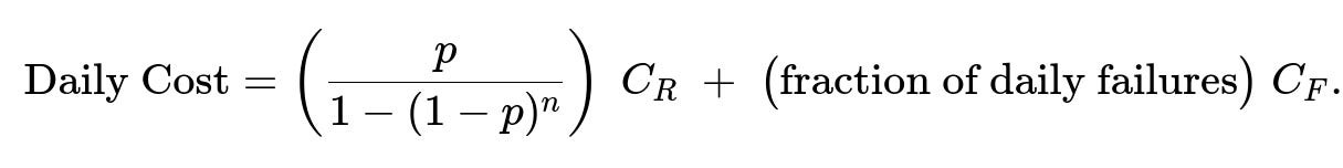
But note that fraction of daily failures is part of the replaced vehicles. If you prefer to break it out, you can multiply the fraction that fails by ( C_F ) and the fraction that is replaced from forced replacement by ( C_R ). The fraction replaced daily is from both failures and forced replacements.
You can do an optimization: pick n to minimize overall cost. For a given n, the fraction replaced daily is ( x_0 ). You can also consider if investing in reliability reduces p at some cost. Then you have a multi-variable optimization problem:
Decide n (how long to keep vehicles).
Decide how much to spend on reliability improvements that reduce p.
Pitfalls:
Some cost components may not be linear in p or in the fraction replaced (e.g., large disruptions if many vehicles fail simultaneously).
You might have constraints, such as you cannot choose n beyond a certain limit due to regulatory or safety rules.
p might not be purely under your control; real reliability improvements might have diminishing returns or practical limits.