ML Interview Q Series: Steady-State Vehicle Replacement Rate via Expected Lifetime with Daily Failure Probability.

Browse all the Probability Interview Questions here.

32. Suppose there is a new vehicle launch upcoming. Initial data suggests any given day has probability p of a malfunction or crash requiring replacement. Additionally, any vehicle that has been around n days must be replaced. What is the long-term frequency of vehicle replacements?

Answer Explanation and Derivations

Understanding the Problem and Key Ideas

The scenario involves vehicles that can fail (or crash) on any given day with probability p. Once a vehicle crashes, it must be replaced immediately. Additionally, there is a policy that no vehicle can operate longer than n days, so if a vehicle survives up to day n, it must be replaced at that time anyway.

In the long run, there will be a large population of vehicles, each in different “ages” of their lifespan. We assume every new or replacement vehicle starts at “day 1 of usage,” then day 2, and so forth, until it either fails with probability p on one of those days or reaches day n and gets replaced regardless of whether it would fail on that day. We are interested in finding the fraction of vehicles that are replaced on a typical day, in a steady-state sense.

Key Points About the Replacement Rate

Each vehicle’s random lifespan can be viewed as the minimum between a geometric random variable (with success probability p, describing when it crashes) and a fixed cutoff day n. If we call the lifespan random variable X, then X takes values from 1 to n, where:

The probability a vehicle fails exactly on day k (for k from 1 to n - 1) is the probability it survived the previous k - 1 days and fails on day k. If the vehicle reaches day n without failing on days 1 through n - 1, it is replaced on day n anyway (forced replacement).

Once we compute the expected lifetime E[X] in days, the long-term fraction (rate) of daily replacements is the reciprocal of that expected lifetime. The intuition is that if vehicles on average last E[X] days, then each day we replace about 1/E[X] of the entire large pool of vehicles in the steady state.

Mathematical Expression for Expected Lifetime

Let X be the lifespan of a single vehicle. Define q = 1 - p as the probability that a vehicle survives (does not fail) on a given day. Then:

The probability that X = k for k = 1, 2, ..., n - 1 is

because it must survive the first k - 1 days and fail on day k.

The probability that X = n is

because it must survive all days 1 through n - 1, and then it is replaced on day n (regardless of whether it would fail on that day).

Hence the expected lifetime E[X] can be written as a sum:

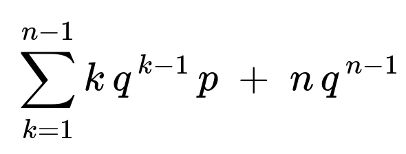
Because q = 1 - p, this expression accounts for all possible days k from 1 to n - 1 on which a crash happens, plus the forced replacement day n if the vehicle survives that long.

Long-Term Frequency of Replacements

Once we know E[X], the fraction of vehicles replaced in the long run per day (in an approximately steady-state system) is:

Therefore, the long-term frequency is the reciprocal of the expected number of days a vehicle remains in service before replacement. Substituting the sum from above, the frequency is:

This formula captures both the effect of random daily crashes with probability p and the mandatory replacement after n days.

Practical Implementation and Simulation Example

It can help to confirm this analytical result by writing a quick Python simulation that empirically estimates the fraction of daily replacements in a large simulated fleet. Below is a brief example.

import numpy as np

def simulate_replacements(num_days=10_000_00, p=0.01, n=50):
    # Track total vehicles replaced. We assume we start with a large number
    # of vehicles, each with a random "day of age" from 1..n to emulate steady state.

    # For simplicity, let's just track a large array of current ages for vehicles.
    # Then we step day by day, increment ages, apply crash probability, and forced replacement.

    fleet_size = 10_000_00  # large number of vehicles
    # Initialize random ages so that we start in approximate steady state
    # (this is not a perfect steady state start, but close enough for demonstration).
    ages = np.random.randint(1, n+1, size=fleet_size)

    total_replacements = 0

    for _ in range(num_days):
        # Vehicles that crash
        crashes = np.random.rand(fleet_size) < p
        # Vehicles that hit day n
        forced = (ages >= n)

        to_replace = crashes | forced  # logical OR
        total_replacements += np.sum(to_replace)

        # Replace those vehicles with new ones age=1
        ages[to_replace] = 1

        # For the rest, increment age
        ages[~to_replace] += 1

    # Average daily replacements over the simulation
    return total_replacements / num_days

p = 0.01
n = 50
empirical_rate = simulate_replacements(num_days=100000, p=p, n=n)
print("Empirical replacement rate:", empirical_rate)

By comparing empirical_rate with the analytical formula 1 / E[X], we can verify they agree for large simulation runs.

Potential Edge Cases

It is useful to check extreme values:

If p = 0, the vehicles never fail except for the forced replacement at day n. So every vehicle lasts exactly n days, and the expected lifetime is n. The long-term replacement frequency is 1 / n. If p = 1, then vehicles fail every day with certainty. None of them ever reach day 2. So the expected lifetime is 1, and the replacement frequency is 1. If n = 1, every vehicle is replaced after a single day no matter what, because either it fails on that first day or it is forced out anyway. That also yields a frequency of 1.

These checks match intuition and confirm that the formula behaves appropriately in boundary conditions.

What if we want a closed-form expression for E[X]?

A closed-form expression can be derived by summing partial series, but the form given by the summation is typically straightforward enough and easily computed numerically. If needed, one can use known series expansions for sums of the form

which relate to geometric series derivatives, but in practice the direct summation is usually fine for large n, especially in code.

How is the result used in real-world fleet management?

The formula allows management to estimate on average what fraction of the fleet will need replacing each day. This is crucial for logistics, spare parts planning, and manufacturing capacity. If the fraction is too high, the system might need to investigate ways to lower p (improve reliability) or extend n (reduce forced replacements). However, extending n might not be feasible in some strict safety or regulatory contexts, so the only option is to reduce the daily crash probability p.

How would you handle correlation or varying failure probabilities over time?

If the failure probability is not constant but changes with vehicle age, environment, or usage conditions, the analysis would need to be adjusted. One might define p_k as the probability of failing on day k. Then each day’s survival probability changes accordingly. The forced replacement at day n would still apply. The expected lifetime formula and the final replacement fraction would be generalized by summing over all possible day-dependent crash probabilities.

How do you handle partial day usage or continuous-time hazard rates?

If the process were modeled in continuous time with hazard rates, we could integrate an appropriate survival function up to time T (the continuous analog of day n) and also incorporate the forced replacement time. The discrete-time approach here is a simplified version of that. But the essence remains: you compute the expected usage time and take its reciprocal for the daily fraction replaced in steady state.

Are there cost implications that can be linked to this replacement rate?

In a real business, you could multiply the daily fraction replaced by the cost of each replacement to get average daily replacement cost. You could also incorporate intangible costs such as downtime or brand damage if these crashes happen on the road. Some advanced models might attempt to minimize a combination of manufacturing costs, maintenance costs, and safety risk, subject to constraints on how many crashes are acceptable.

Are there special techniques if data on failures is limited?

If p is uncertain, you can place a Bayesian prior on p and update it as you observe actual daily failures. That approach is common when there are not many historical data points. Once updated, you can re-estimate the expected lifetime and daily replacement fraction.

Could you solve the problem by focusing on steady-state age distribution?

Yes, you can also reason that in steady state, a fraction of vehicles are in “age 1,” “age 2,” and so on, up to “age n.” You can solve for the proportion in each age class, then sum the fraction that fails or is forced out on each day. That approach leads to the same result. It may also help in more complex setups where p depends on age.

When you compute that fraction in each age, let π_k be the steady-state proportion of vehicles that are exactly k days old. You can form equations based on how vehicles flow from age k to age k+1 (minus those that fail or get replaced). Solving that system yields the same final replacement fraction. The approach with expected lifetime is often simpler, but both methods confirm the same answer.

What is the final succinct statement of the solution?

The daily long-term replacement fraction is the reciprocal of the expected vehicle lifetime. The expected lifetime is computed by summing over all possible outcomes: fail on day k (for k=1 to n-1) or make it to day n and be replaced. The resulting formula is:

Below are additional follow-up questions

Could forced replacement at day n interfere with performing reliability analyses on the vehicle?

Forced replacement at day n can complicate reliability analyses since the vehicles do not run beyond n days. In typical reliability studies, you want data on how long a system truly lasts under normal or stressed conditions. Because any vehicle reaching n days is removed regardless of whether it would have continued functioning longer, the data is right-censored at day n. This makes it harder to characterize the underlying distribution of failures, especially if the forced replacement day is well before many natural failures would have occurred.

In a practical setting, if you want accurate estimates of inherent reliability separate from forced replacement policies, you need to collect data on actual failures independently of whether day n has arrived. You might run a small test fleet without forced replacement, or extend n in controlled conditions, to observe genuine time-to-failure. Alternatively, you can treat the data as censored at day n and use survival analysis methods to account for that right-censoring. A potential pitfall is that if you do not properly account for censoring, you could underestimate or overestimate the actual crash probability.

In real-world scenarios, an organization might set n to mitigate risk—perhaps certain critical components are deemed unsafe after a certain time. But this does limit the amount of data you get on later lifetimes. So it is essential to keep in mind that the forced replacement imposes an artificial boundary on any lifetime measurements.

How does the replacement rate change if we consider partial failures or events that trigger servicing but not full replacement?

In reality, not every malfunction leads to a total replacement. Sometimes a vehicle malfunction may be repairable. The model presented assumes a single daily probability p of a malfunction requiring total replacement, which is a simplified premise. If partial failures occur frequently but do not mandate replacement, the fraction of total replacements could be lower.

A refined approach might assign probabilities to different severities of malfunction:

1. Minor failures (vehicle is repairable, does not require full replacement).

2. Moderate failures (vehicle is out of service for a certain number of days for repairs).

3. Major failures (vehicle must be replaced).

You would then incorporate these probabilities into a Markov chain or survival analysis with competing risks:

• Probability p_major that a failure is irreparable, leading to immediate replacement.

• Probability p_minor that a failure is repairable (the vehicle returns to service after some downtime).

• Probability 1 - (p_major + p_minor) that there is no failure on that day.

The forced replacement after n days still applies. The steady-state fraction of replacements would then be 1 / E[X], where X is the random lifetime that ends specifically in major failures or forced replacement. Minor failures would only affect the lifetime distribution if they somehow accelerate wear or reset the “clock,” depending on the system design. A subtle pitfall is mixing up all downtime events (minor plus major) with actual replacements, which leads to inaccurate estimates if not carefully distinguished.

What if the crash probability p depends on usage intensity, and usage intensity changes over time?

In many real fleets, the daily crash or failure probability is not constant. It might be higher on weekends (if usage is more intense), or vary with road conditions, weather, or seasonal demand. If p depends on external factors, then the single constant p used in the formula is not strictly correct. You might need a piecewise definition or function p_t representing the day’s environment. Over the course of a year, you could have different probabilities each day.

One approach is to compute an “effective p” if usage is relatively stationary on average, but that loses the nuance of day-to-day variance. A more accurate method would define a day-dependent probability p_t. The lifespan distribution then becomes more complex to compute analytically, but you can still model it in a simulation:

1. Each day, a vehicle “age” increments.

2. The fail probability on day t depends on external context (p_t).

3. Forced replacement occurs at day n regardless.

The pitfall is that you can no longer simply say the daily replacement fraction is 1 / E[X] with X derived from a single p, because the underlying probability changes over time. Nonetheless, you can still simulate a large fleet under the varying p_t scenario to estimate the steady-state fraction replaced. Or you can carefully sum up the probabilities across each day of the vehicle’s potential life, but the result is a bit more involved mathematically.

In practice, could the replacement day n align with scheduled maintenance intervals?

Yes. Often, industrial fleets schedule major maintenance at fixed intervals—for instance, every n days or every n miles. The forced replacement might be aligned with these intervals if the cost of refurbishing or overhauling is significant enough that total replacement is more economical. However, misalignment might occur if the forced replacement schedule (set for safety reasons) is different from the typical maintenance interval. You might end up with vehicles that get replaced prematurely relative to their next major scheduled maintenance.

A subtle real-world consideration is whether forced replacement truly replaces the entire vehicle or just major components. You might have partial refurbishments or rebuilds that effectively reset the “age” of certain parts but not the entire system. Then you have to define carefully what “day 1” means. If the forced replacement involves the entire vehicle, the model is straightforward. If it only involves certain assemblies, the overall risk profile changes in ways that are more complicated to track.

Could backlog or supply chain delays affect the interpretation of the replacement rate?

If there are supply chain bottlenecks, the vehicle might fail (or reach day n) but not be replaced immediately because new vehicles are out of stock. This would create a lag between when a vehicle becomes inoperable and when it re-enters the fleet as a newly replaced vehicle. The basic mathematical model assumes immediate replacement—there is a one-to-one transition from a failed vehicle to a new one.

In reality, if replacements are delayed, you may have fewer total vehicles operating on the road. Over time, the fraction of in-service vehicles replaced might remain the same once a steady state is re-established, but there could be a queue or waiting time for new vehicles. One pitfall is ignoring the downtime cost. If you rely on a certain fleet size for operations, the daily fraction replaced is not the whole story; you also need to factor in how quickly a replacement can be procured. In high-volume industries, large surge demands for replacements might cause short-term disruptions that are not captured in a simple average replacement fraction.

How would you adjust the model for vehicles that get replaced only if the cost of repairs exceeds a threshold?

In practice, companies sometimes choose to repair vehicles unless the cumulative repair cost (or single-event repair cost) surpasses a certain threshold, at which point the vehicle is replaced. That threshold-based approach creates a more nuanced decision rule. The probability p in the original model can be seen as the “probability that a failure is beyond repair threshold.” However, if repairs are frequently cost-effective, p effectively shrinks because not every failure leads to immediate replacement.

You might generalize the daily crash probability to:

• Probability p_fail that some failure happens.

• Conditional probability p_replace|fail that a failure leads to replacement (due to cost threshold).

Then the effective daily probability of a replacement is p_fail * p_replace|fail, along with forced replacement at day n. Additionally, you might incorporate dynamic usage: if the vehicle has had repeated repairs, the threshold might be lower or the risk might be higher. An important pitfall here is double-counting or incorrectly mixing major and minor failure events if you do not carefully separate them in the model. You must define whether repeated failures are correlated with increased future breakdowns, which complicates the independence assumption in the simple daily crash model.

How do you handle multiple forced replacement conditions, for example both day n and mileage m?

Some fleet policies specify maximum operating life in terms of calendar days or total miles driven. If either threshold is reached, the vehicle is replaced. This effectively adds a second dimension: time in service and usage (miles). The probability of failing on any given day might also be a function of total miles traveled. You could model it with a bivariate distribution tracking (day, total_miles).

Every day, vehicles accumulate some expected miles. A forced replacement occurs if the day count hits n or the total miles hits m, whichever comes first. In parallel, a daily failure event can happen with some probability that might also depend on total miles or vehicle age. The straightforward approach is once again simulation, or you can attempt more advanced reliability modeling using hazard functions that incorporate both time and mileage. One subtlety is that different vehicles might be driven different amounts daily, so you may not have a single usage rate for all. This can greatly complicate analysis, because the forced replacement mileage might come sooner for heavily utilized vehicles, whereas lightly used ones might hit the day threshold first.

What if there is a warm-up period where the probability of failure is higher initially?

Some complex mechanical systems have what is called “infant mortality,” where brand-new parts might have defects that cause a higher failure rate early in life. Over time, the vehicles that survive that early period tend to have a lower failure rate until old age sets in, and then the failure rate increases again. This is often visualized as a “bathtub curve.” The daily constant p in the simple approach does not capture that shape.

If you want to integrate a higher failure probability in the first few days, then a lower probability for the middle portion, and eventually an increasing probability near the end of life, you would break it down: p_k depends on k, with a certain distribution. The forced replacement day n still applies. The average lifetime E[X] would be computed with the day-dependent probabilities. A pitfall is to ignore the possibility that some fraction of vehicles fail extremely early due to manufacturing defects, skewing the distribution. Another subtlety is that scheduled maintenance or improvements might reduce the risk in certain phases, so the shape of p_k might change if you do mid-life inspections or part replacements.

Does the result hold if the system is not yet in steady state?

The formula for the fraction of vehicles replaced each day (1 / E[X]) describes a steady-state scenario, assuming a large, stable fleet where vehicles are continually being replaced in the same distribution. If the fleet is new, you have an initial population of vehicles all at age 0 (or age 1) on day one. Early on, the replacement rate might not match 1 / E[X] because the age distribution of vehicles is concentrated at the low end.

Given enough time, though, the fleet approaches a steady-state distribution of ages, unless there are large expansions or contractions in the total fleet size. A subtle pitfall is analyzing data from an early rollout and concluding the replacement fraction is smaller or larger than the long-run fraction. Practically, a company might see very few replacements in the first few weeks of a brand-new product (especially if p is small and n is large). Over months or years, though, the 1 / E[X] formula is expected to hold more accurately once the system stabilizes.

Could the environment or usage change drastically after day n is chosen, making the model assumptions invalid?

Yes. Suppose day n was selected based on historical data, but after introduction of a new feature or a shift in usage patterns, the daily crash probability p changes. Or the usage environment shifts from mild climates to more harsh operating conditions. The forced replacement day n might be suboptimal for the new environment, or the estimated daily failure probability might no longer be accurate.

The pitfall is that relying on stale assumptions can produce a mismatch between predicted and actual replacement rates, possibly leading to either overstock or shortages of replacement vehicles. A forward-thinking strategy is to continuously monitor actual failures, re-estimate p (or a distribution of p_k), and then reevaluate if n is still appropriate. If you see a higher crash rate than expected, you might lower n. Alternatively, if vehicles are performing better than forecasted, you could extend n to reduce replacement overhead.

What if there’s a cost model that balances forced replacement day n with daily failure cost?

Often, the choice of n is an optimization problem. Replacing vehicles too early wastes resources if they still have a relatively low probability of failure. But waiting too long may cause more frequent (and possibly more expensive) failures. If you incorporate costs, you might define:

• C_rep: cost of replacing a vehicle.

• C_fail: cost of a failure event (including downtime, repairs, damage, etc.).

In a day-based model, you want to minimize expected total cost per vehicle over its lifetime:

• Probability p of a failure event each day (with cost C_fail).

• If the vehicle reaches day n, forced replacement (cost C_rep).

• If it fails earlier, also cost C_rep to replace.

You could set up an expected cost equation as a function of n. Then, you choose n to minimize that cost. This is more complex than the original question, but a real-world pitfall is ignoring how large the failure cost might be or how it might escalate with repeated failures. In an extreme scenario, if a catastrophic failure is extremely costly (C_fail is huge), you might choose a smaller n to avoid that risk. Conversely, if C_fail is small or you have good insurance coverage, you might find a larger n is more cost-effective.

How would dependencies among vehicles affect the replacement rate?

If vehicles operate in a network, one vehicle’s crash might affect others (e.g., a multi-vehicle accident). This interdependence can cause correlated failures that are not captured by a single independent daily probability p. If a crash by one vehicle significantly increases the chance of crashes in the same region or fleet, you need to model those correlations. In that case, the fraction of replacements on a given day might cluster or vary significantly day to day. A naive model that assumes independence would underestimate the risk of simultaneous replacements.

Another possibility is that forced replacements might happen in batches if a design flaw is discovered, prompting a recall. In that event, you might see large spikes in replacements unrelated to the daily p. This batch effect is a pitfall if you rely on an independent daily crash probability. Realistically, a manufacturer recall due to a discovered defect can overshadow the normal p-based replacement model.

Are there any complications if vehicles are not identical?

A homogeneous fleet assumption—that all vehicles have the same p and the same forced replacement day n—might be too simplistic. Real fleets can comprise multiple vehicle models, each with different reliability profiles. If half the fleet is an older generation with a higher failure probability, and half is a newer generation with a lower failure probability, you must segment them or use a weighted approach. The forced replacement policy might even differ by model (some might allow longer usage if reliability is proven to be higher).

A subtle pitfall is averaging everything into a single p and single n, which could mask the fact that certain models are far less reliable and drive up overall failures. In practice, you could define p_i and n_i for each model or each technology generation. Then you might track or simulate the overall fraction of replacements. This results in a more complex but realistic multi-population approach. You also might do policy changes—like forcing earlier replacement for less reliable models or extending usage for proven new models.

How could software updates or incremental improvements during a vehicle’s lifetime factor in?

Modern vehicles often receive frequent software updates that can significantly alter their reliability over time. A safety-critical patch might decrease the crash probability p. Alternatively, a buggy update might momentarily increase p. The forced replacement day n might stay fixed, but effectively the daily crash probability changes because the underlying software/hardware changes. Another scenario: the manufacturer might recall or replace certain components mid-lifecycle to reduce the probability of failure.

These factors dynamically shift p in ways that might be difficult to predict at the time the policy is set. One pitfall is not accounting for downward trends in p if software improvements effectively reduce the failure rate, thus leaving n suboptimally low. Or, if an unexpected bug emerges that raises p significantly for vehicles in certain conditions, the forced replacement day might need revision. In practice, continuous monitoring and re-estimating p over time is critical for aligning the forced replacement threshold with real reliability data.

What if there’s a limit on how many vehicles can be replaced in a single day?

If the system cannot process unlimited replacements in a single day—maybe there is a cap on manufacturing capacity or the logistical system can only handle a certain throughput—then on days when more vehicles fail than can be replaced, some vehicles may stay out of service. This leads to a backlog. Over time, an equilibrium might still form, but it’s no longer correct to say the fraction replaced daily is just 1 / E[X]. Instead, the daily replacement fraction would be capped, and vehicles that fail would remain in the queue until they can be replaced.

A potential real-world pitfall is ignoring the queue or backlog effect and incorrectly assuming an unlimited replacement pipeline. During times of higher-than-expected failures, your actual replacement fraction might be suppressed by that capacity constraint, causing operational disruptions and unsatisfied demand. Eventually, you might see day-to-day variations in replacement rates as the backlog is resolved. In advanced settings, you could incorporate queue theory or dynamic simulation to handle that constraint.

What is the significance of random vs. deterministic usage patterns across different fleets or regions?

In some fleets, usage is fairly deterministic, with each vehicle running the same route daily. In others, usage can vary widely among vehicles (e.g., some might idle for days, others might run 24/7). The daily crash probability p could differ drastically across vehicles or days. The simpler model lumps everything into a single p, which might be seen as an “averaged” probability. But if there is wide dispersion, the actual distribution of lifetimes can deviate from a simple geometric model.

One might try to break the fleet into categories: high-usage, moderate-usage, and low-usage vehicles, each with its own p value. Then you can compute an expected replacement rate for each category and sum them up, weighting by the fraction of vehicles in each category. The subtlety is ensuring you have accurate data on how usage patterns translate to failure probabilities. If usage data is incomplete or not well-tracked, you might incorrectly set p, leading to forecasting errors.

Once you start combining categories, the forced replacement day n might also differ across them (perhaps high-usage vehicles have a smaller n because they wear out more quickly). That creates a piecewise approach to modeling the entire fleet’s replacement fraction.

How does random sampling variability affect estimation of p from real data?

In practice, p is estimated from observed crash events. If the underlying true daily failure probability is small (e.g., p < 0.001), you might need extensive data to estimate it accurately. Small-sample noise can lead to wide confidence intervals around your p estimate. This in turn affects your estimates of the daily replacement fraction. If you pick p too high because of a small sample with an unusually large number of early failures, you may overestimate the fraction replaced and overstock on replacements.

A subtlety is that real data can exhibit overdispersion or cluster effects—failures might bunch up in time due to external factors. Traditional binomial or geometric assumptions might not precisely fit. Thus, one pitfall is ignoring the possibility that your observed short-term data is not representative of the true long-run probability. Practically, you might incorporate confidence intervals for your replacement forecasts, track usage conditions, and continually update your estimates as more data arrives.

Would partial solutions, like only forcing replacement on certain critical components, change the model?

Sometimes, rather than replacing the entire vehicle at day n, you might replace or overhaul critical systems (e.g., the battery in an electric car, or the engine in a traditional vehicle). If that drastically reduces the risk of failure, you can effectively “reset” the lifetime for the critical component. But other components might still fail. This partial replacement policy modifies how you define a “vehicle,” because you might keep the same shell but replace the key subsystem. The forced replacement day for that subsystem might differ from the rest of the vehicle.

A potential pitfall is ignoring that partial replacements can yield a new distribution of daily failure probabilities after the component swap, rather than continuing with the old probability. In real fleets, some managers treat a major subsystem replacement almost like having a new vehicle, especially if the replaced component is the primary source of failures. But to fully model this, you’d need a multi-phase approach:

• Phase 1: Probability of failure prior to subsystem replacement.

• Phase 2: Probability of failure after subsystem replacement.

Even if you keep the same overall day n, each subsystem might have its own forced replacement schedule or indefinite usage if it’s recently replaced. This is no longer a simple one-parameter daily crash probability model.

Could external events or recall campaigns temporarily increase the forced replacement rate outside the day n policy?

Yes. If a manufacturer issues a recall, you might have a sudden spike in replacements, especially if the recall affects vehicles of a certain vintage or that exhibit a certain issue. This forced replacement might happen independently of whether a vehicle has reached day n or not. It creates an extra mechanism for removing vehicles from service. That means your actual daily fraction replaced can spike above what the p-based model predicts.

Ignoring these events can produce large deviations from the theoretical replacement fraction. A real-world fleet manager must treat recall-driven replacements as additional forced replacements. In a day-based model, you could treat them as random “shock” events that occur rarely but affect many vehicles at once. Estimating the long-run fraction replaced still might average out to the original formula if recalls are extremely rare, but if recalls happen with any frequency, they can significantly inflate the overall replacement rate.

Are there any security or regulatory considerations that could prompt forced replacements sooner?

In certain industries (aviation, defense, autonomous vehicles), regulators might mandate a maximum operating duration if new safety data emerges. If n is lowered abruptly—say from 60 days to 30 days—then vehicles at ages between 31 and 60 may all be forced out simultaneously. This disrupts the steady-state assumption. After the transition, a new steady state might form around the new n. A pitfall is failing to anticipate potential regulatory changes. If the environment is highly regulated, you might see multiple forced replacement thresholds over time, each requiring re-analysis of the daily replacement fraction.

In real-world contexts, a best practice is to maintain flexible models or simulations that can recalculate the expected replacement rate quickly for any new n mandated by regulators. Additionally, if crash data or near-misses reveal that p is higher than initially thought, regulators might force shorter intervals to reduce risk, further increasing your daily fraction replaced.

Could the model be extended to track not just replacements but how many vehicles are active in the fleet each day?

Yes. The question focuses on the fraction of vehicles replaced daily, but you might also be interested in how many vehicles remain in service at each point in time. By combining the daily replacement fraction with new additions to the fleet (if the fleet is expanding) or retirements (if the fleet is shrinking overall), you can track the total active vehicles. In a stable scenario with neither expansion nor contraction, the total active vehicles might remain approximately constant, with new replacements balancing out the older vehicles that crash or age out.

If you are in a growth phase—buying new vehicles faster than they are failing—then the fraction replaced daily might remain similar, but the absolute number of vehicles replaced daily grows. A subtlety is that the fraction can remain stable even as the absolute count changes drastically. In large expansions, it takes longer to reach a steady state of age distribution. One might do a time-based simulation to see how quickly the age distribution converges to a steady pattern when the fleet is ramping up.

Can environmental or usage variation among days push the model outside Markov chain assumptions?

Yes, if you assume a memoryless Markov chain with daily probability p of failure, you are implying that each day’s survival does not significantly alter the next day’s failure risk (beyond incrementing age up to day n). If environmental factors or usage patterns on day k affect the probability of failing on day k+1 in a way that goes beyond simple increments of age, then the Markov chain assumption is violated. For example, intense operation on day k might accelerate wear and greatly increase the next day’s probability of failure.

A pitfall is applying the simpler model to a domain with strong day-to-day dependencies. The daily probability p might no longer be memoryless. Instead, you might have to define a more complex state, such as the internal wear level of the vehicle, or use a Bayesian updating process that increments failure probabilities based on the stress experienced. This leads to a more complex model, and the forced replacement day n remains an external boundary condition. In such cases, the neat formula for the daily replacement fraction might only be an approximation, or you must run simulations that incorporate the dynamic hazard rate.

Does the conclusion still hold if partial usage days are counted differently?

Sometimes a vehicle that runs only half a day might be considered “half usage,” leading to a different forced replacement policy measured in total operational hours. The day-based model might treat it as a full day even if the vehicle is used only part of the day. This can distort the data if the usage pattern is variable. For example, a vehicle used for only a few hours daily might be replaced exactly at the same day n as a vehicle used for 24 hours daily, which might be unfair or suboptimal.

One approach is to measure vehicle age in total operational hours (or total distance traveled) rather than calendar days. Then the forced replacement is after n hours or n miles. The probability p can be reinterpreted as a per-hour or per-mile failure probability. But that changes the entire parameterization of the problem. If you keep the day-based approach, be mindful that partial usage can artificially compress or extend the actual usage period relative to the forced replacement day. A real pitfall is ignoring how partial usage might systematically reduce failures while still applying the same replacement schedule.

How does the model handle repairs that might happen even if there’s no crash?

Some fleets perform preventative maintenance or repairs to fix minor issues before they become major. Although these do not cause replacement, they might improve reliability, potentially lowering the daily failure probability p for subsequent days. So p might not be truly fixed. Alternatively, if a vehicle experiences repeated minor repairs, the operator might choose a replacement earlier than day n to avoid further downtime. That leads to a separate policy-driven forced replacement that is not strictly day-based but triggered by cumulative repair events.

A pitfall here is mixing up a purely random daily crash probability with a structured preventative maintenance program. In reality, a well-designed maintenance program might reduce p substantially for vehicles that have been serviced recently. Or it might extend the effective lifetime beyond n if the policy allows skipping the forced replacement if a thorough overhaul is performed. If the day n policy is absolute, maintenance might not change the day-based forced replacement, but the operational daily crash probability might be altered. Accurately modeling this requires capturing the maintenance effect on reliability.

Could random spikes in p due to external crises (e.g., severe weather, road closures, labor shortages) temporarily raise the replacement fraction?

Yes. In severe weather conditions, more vehicles might crash, effectively increasing p for a short period. If that leads to a spike in daily failures, then the fraction of vehicles replaced that day can surge, even though the average fraction might remain around 1 / E[X] over the long run. Realistically, you could see day-to-day volatility around that average. When you compute a long-term average, these spikes average out if they are infrequent. However, if severe events become frequent, the average daily fraction might drift higher than the original estimate.

A real-world pitfall is planning capacity based only on the mean fraction replaced, ignoring the short-term variability from events like storms, large accidents, or labor disruptions. Organizations that need to guarantee continuous operations might plan for surges in demand for new vehicles, so they stock spares or have an expedited manufacturing line for emergencies. If you rely purely on the stable 1 / E[X] figure, you may be caught off-guard by these spikes.

How do you handle regulatory constraints or ethical considerations about the acceptable daily crash probability?

Even if you can mathematically calculate that the replacement rate is 1 / E[X], certain industries might impose limits on how many vehicles can fail daily due to safety or ethical concerns. If p is too high, you might face pressure to reduce daily usage or implement stricter forced replacement intervals. In an autonomous vehicle context, a daily crash probability of p might be unacceptable if it leads to too many accidents. Instead of optimizing cost, the overarching priority might be to reduce crashes below a certain threshold. That might imply drastically lowering n or improving design to reduce p significantly.

A subtle issue is that the forced replacement day n might not fully mitigate safety concerns if p is still large in the early days. Ethical or regulatory bodies could require a more advanced approach, such as a real-time telemetry system that monitors vehicle health to dynamically retire vehicles if they show signs of impending failure. This approach is more advanced than the basic daily probability p model but is often used in industries where safety is paramount (e.g., aviation).

Does the forced replacement policy imply we ignore the possibility that older vehicles might have a higher daily probability of failing?

Yes, if we set a single daily probability p and a forced replacement day n, we are implicitly assuming a fixed failure probability on each day that the vehicle is in service. That might be an approximation if in reality the failure probability changes with age. The forced replacement day n might be chosen specifically because beyond n days, the risk grows unacceptably high. But if the risk does not significantly rise until day n is reached, then p might be fairly constant in the earlier days. Alternatively, if the risk grows gradually, you might be overestimating or underestimating daily failures by using a constant p.

Hence, a pitfall is that the actual daily hazard might be function of k, the vehicle age. If so, the formula for E[X] changes. The key idea remains that the fraction replaced daily in steady state is 1 / E[X], but you must compute E[X] using the age-dependent p_k. If someone uses the simpler model incorrectly when p is truly not constant, they might get the wrong fraction replaced. Real data might show more or fewer replacements than predicted. This discrepancy can reveal that p is not actually constant.

Could user behavior or operator training significantly affect p?

Yes. Suppose the manufacturer invests in better operator training that reduces crash rates. Over time, that lowers p. The forced replacement day n could stay the same, but the fraction of vehicles replaced daily from crashes would drop. In a large fleet, as operators become more skilled, the forced replacements might increasingly dominate the total replacements, eventually overshadowing crash-based replacements.

The pitfall is that if you treat p as a purely mechanical reliability factor, you ignore the human element. In some fleets (like trucking or delivery services), driver skill or compliance with safety protocols is a big determinant of accidents. Proper training, route planning, or telematics can reduce p significantly. Hence, a real-world solution might focus more on lowering p than adjusting n, because a high p is costly and dangerous. Conversely, if user behavior worsens (e.g., new drivers or more aggressive driving), p can jump higher than the original estimate, leading to an unexpected spike in replacements.

What if vehicles are leased, so replacements might occur at the end of a lease rather than day n?

In some industries, fleets are leased for a fixed term (e.g., 36 months). On lease termination, the vehicle is either returned or replaced, possibly ignoring whether it’s day n in a daily sense. That is effectively a forced replacement, but it might not align with an n-day usage cycle. If the day-based forced replacement policy also exists, you have two conflicting triggers: day n or the end of the lease, whichever comes first.

A hidden complexity is that the daily crash probability p might remain the same, but you have a different forced replacement schedule driven by contractual obligations. The combined forced replacement might effectively yield a smaller “maximum usage duration” than n. The subtlety is that if the lease term is shorter than n, the forced replacement day n might never be reached for a large fraction of vehicles. In that case, the fraction replaced daily is dominated by either lease returns or crashes. You could unify them in a single approach by defining the forced replacement day as min(n, lease_length_in_days). Still, you must ensure your data on p is relevant to that shorter timescale.

If we keep adding features that incrementally raise or lower p, how do we keep the model accurate?

Vehicles often evolve with software and hardware changes. Every time a new feature is introduced (such as improved collision-avoidance sensors), the effective daily crash probability might shift. Maintaining an up-to-date model requires reevaluating p for vehicles with the new feature. The forced replacement schedule might remain the same, but the distribution of times to failure changes. Over time, you might end up with multiple sub-fleets: older models with higher or unknown p, and newer models with improved or tested p. The manager might want an overall daily fraction replaced across the entire fleet.

One subtlety is that short pilot programs might not yield enough data to confidently estimate p for the new feature, so you might rely on older data or limited trials. That in turn can lead to miscalculation of the expected daily crash rate in production. Thorough testing and a phased rollout strategy can help reduce uncertainty. Another pitfall is that older vehicle data might become misleading as soon as a new sensor or system significantly changes reliability. You should either run separate models for new vs. old vehicles or find a bridging method to unify them.

How would changes in day length or operational hours shift the n-day policy?

In some industries (e.g., mining, offshore operations, or polar regions), the concept of a “day” can vary with extreme latitudes or rotating shift schedules. If “daily usage” is not consistent—some days might be 24 hours of operation, others might have partial usage—it might be more accurate to adopt “operational cycles” or “hours of operation” as the unit for forced replacement.

If the forced replacement policy is strictly in calendar days, but the actual usage is cyclical or partial, you might end up replacing vehicles at times that do not align with actual wear and tear. For instance, if you have continuous usage in a 24/7 operation, each “day” is far more usage than for a vehicle used normally for 8 hours. This mismatch can produce suboptimal scheduling or inaccurate estimates of failure. A deeper approach uses usage-based or cycle-based metrics rather than pure calendar days.

Does insurance cost factor into the forced replacement policy?

In many fleets, the operator pays insurance, and the insurance rate might escalate with vehicle age or usage. If older vehicles are seen as riskier, insurance might become prohibitively expensive after day n. That can lead the fleet manager to adopt a forced replacement policy earlier than the mechanical reliability threshold. This adds an economic dimension to the replacement decision. The daily crash probability p is still relevant, but the overall cost function might say: “Even if p is not too high, insurance costs become unsustainable after day n, so we must replace.”

A pitfall is ignoring the influence of insurance or compliance costs on replacement policies. If you rely purely on mechanical or reliability-based arguments, you might set n too high, never factoring in that the insurer might drastically raise premiums, overshadowing any cost savings from extended usage. Conversely, a heavily subsidized or self-insured operation might be able to push n further without incurring major insurance penalties, so the mechanical reliability model might remain the main driver.

Are there any hidden assumptions about immediate detection of failures?

The standard approach presumes that when a crash or failure occurs, it is immediately recognized that the vehicle must be replaced. In reality, certain failures or malfunctions might be detected only after an inspection or once a driver reports an issue. If detection is not instantaneous, some vehicles might remain in service an extra day (or more) despite having a critical defect. That is especially possible if sensors or feedback loops are incomplete.

The pitfall is that the model’s day-by-day viewpoint implicitly assumes perfect, real-time knowledge of whether the vehicle is operational or not. In a real fleet, delayed detection can lead to continued usage until the next scheduled inspection. This can artificially inflate the average time to replacement beyond what you’d expect if you assume immediate detection. Alternatively, if you’re overly cautious and remove vehicles at the first hint of an issue, you might replace them prematurely, effectively raising the daily fraction replaced. Addressing this requires more nuance in how you define “failure events” and the timeline for their detection.

If the fleet is large but the daily crash probability is extremely small, could we still see a stable replacement fraction?

Yes, large numbers help. Even if p is extremely small (say 0.0001), in a sufficiently large fleet you still observe some daily crashes. Over a long period, the fraction of vehicles replaced daily stabilizes around that rate. The forced replacement day n further ensures that vehicles that never fail still eventually get replaced. However, for smaller fleets, random variability might make the observed daily replacements quite erratic.

A pitfall for small fleets is trying to measure the fraction replaced daily from short-term data. If p is small, you might go many days with zero replacements, then see multiple replacements at once. The average over a very long time might still converge to 1 / E[X], but short-term volatility is high. For large fleets, the law of large numbers smooths out the daily fraction to a stable average.

Does combining multiple random processes (e.g., random crash events plus random forced replacement scheduling) raise complexities in interpretation?

You have two main sources of randomness:

1. Daily crashes (a Bernoulli process for each vehicle).

2. The timing of forced replacements (deterministic day n, but in the presence of random survival up to that day).

These combine to produce a distribution of lifespans. Interpreting an individual vehicle’s outcome might be straightforward—it fails on some day k or reaches day n. But in a large fleet, you must ensure you’re not confusing probability distributions from the ensemble with the outcomes for an individual vehicle.

One subtlety is that some vehicles might appear extremely reliable if they never fail up to day n, while others might fail early. The fraction replaced daily is just the aggregate effect. If you attempt to interpret the fraction replaced as purely from mechanical failure, you’ll forget that some fraction is due to forced replacement. Conversely, if you interpret the forced replacement fraction as separate from overall replacement events, you might double count. The model is consistent if you treat them all as a single process culminating in day k or day n, whichever comes first.