
ML Interview Q Series: Subset Overlap: Expectation and Probability via Linearity and Combinatorics

Browse all the Probability Interview Questions here.
33. Alice and Bob choose their top 3 shows from a list of 50 shows, randomly and independently. What is the expected number of shows they have in common, and what is the probability they have none in common?
Understanding the Problem
This is a probability question involving two independent selections from a set of 50 items. Alice chooses 3 shows out of 50, and Bob also independently chooses 3 shows out of 50. We want two main results:
• The expected number of shows (out of the 3 each has chosen) that both Alice and Bob end up picking. • The probability that they have zero shows in common, meaning none of Alice’s picks match any of Bob’s picks.
Intuition and Core Ideas
The problem has a neat combinatorial structure:
Alice’s choice can be viewed as a random subset of size 3 from the 50 shows. Bob’s choice is another random subset of size 3 from the same set of 50. Because both choices are uniform and independent, each 3-element subset is equally likely for each person.
To find the expected number of matches, a powerful strategy is linearity of expectation. Instead of directly counting the overlap distribution, we define indicator variables that track whether a particular show is chosen by both Alice and Bob, and then sum their expected values. This approach is often simpler than enumerating overlaps directly.
To find the probability of no overlap, we can count how many ways Bob can choose his 3 shows so that they are all different from Alice’s 3 shows. Then we divide by the total number of possible ways Bob can choose his 3 shows. Since Alice’s choice is fixed in the probability conditional sense, it’s straightforward to count how Bob’s selection can avoid all of Alice’s shows.
Detailed Derivation of the Expected Number of Common Shows
One of the most elegant ways to compute an expected overlap is to use indicator random variables.


Hence, the expected number of shows in common between Alice’s and Bob’s top 3 picks is 0.18. This means that on average, they share about 0.18 shows, which is less than a quarter of a single show. Intuitively, this is a small number because each is only choosing 3 items out of a fairly large pool of 50.
Detailed Derivation of the Probability That They Have No Common Show

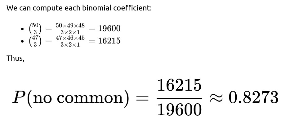
So, about 82.73% of the time, Alice and Bob will not share any show among their top 3 picks.
Implementation Snippet to Illustrate the Concepts
Below is a short Python snippet demonstrating a brute force Monte Carlo check. We can simulate random picks by Alice and Bob many times and empirically estimate both the expected overlap and the probability of zero overlap. This is not needed to prove the result, but it can serve as a sanity check:
import random
import math

def monte_carlo_simulation(num_trials=10_000_00):
    matches_sum = 0
    no_common_count = 0

    for _ in range(num_trials):
        # Randomly choose 3 shows for Alice
        alice_picks = random.sample(range(50), 3)
        # Randomly choose 3 shows for Bob
        bob_picks = random.sample(range(50), 3)

        common = len(set(alice_picks).intersection(bob_picks))
        matches_sum += common

        if common == 0:
            no_common_count += 1

    expected_overlap = matches_sum / num_trials
    probability_no_common = no_common_count / num_trials

    return expected_overlap, probability_no_common

if __name__ == "__main__":
    exp_overlap, prob_no_common = monte_carlo_simulation()
    print(f"Empirical Expected Overlap: {exp_overlap}")
    print(f"Empirical Probability of No Common: {prob_no_common}")
When you run this simulation with a large number of trials, you should see values close to 0.18 for the expected overlap and approximately 0.827 for the probability of no overlap.
Potential Pitfalls and Further Clarifications

Over-counting or Under-counting A common error is to forget the independence or to misapply combinatorial logic if the sets have different restrictions. Here, both choose 3 out of 50 with no further constraints.
Assuming Overlap Always >= 1 Sometimes, people assume it’s quite likely they’ll share at least one show if each chooses 3 out of 50. But the probability of at least one match is actually 1−P(no common)≈17.27%. So in most random scenarios, they do not overlap at all.
Analyzing Expected Value Without Indicators One could try to count all overlaps by enumerating intersection sizes, but that approach is more tedious. The linearity-of-expectation method is much faster and less error-prone.
What if the number of shows was different from 50 or they picked a different number of top shows?
If the total number of shows was n instead of 50, and each person picked k shows, the same reasoning would apply:

Why does linearity of expectation remain valid even if random variables are not independent?
Linearity of expectation does not require independence. Even though each pair (Alice’s picks vs. Bob’s picks) can be correlated across different shows, the expected value of the sum is always the sum of the expected values. This principle holds in general, which is why we can define an indicator variable per show and simply multiply by the probability that both pick the same show.
Could we verify the probability of at least one match?

How does this problem scale for large sets?

Are there any special cases that are worth noting?
• k=1. Then each person picks exactly one show. The probability of a match is 1/n, and the expected overlap is simply 1/n. • k=n. If each picks all shows, the overlap is n obviously, and the probability of no common show is 0. • k=0. Trivial case with no picks from each side. Overlap is always zero.
These edge cases can confirm that the formulas reduce to sensible values when k approaches the boundaries.
Summary of the Final Answers

Below are additional follow-up questions
Q1: How do we compute the variance and standard deviation of the number of common shows?
To analyze the variance of the random variable representing how many shows Alice and Bob have in common, define that random variable as X. We know that

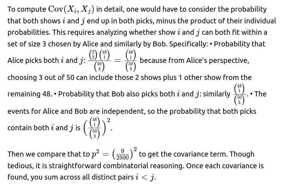
In practical terms, because p is quite small (9/2500), the pairwise correlations tend to be small, so X is dominated by near-independence, but not perfect independence. As an alternative approach, you can estimate the variance via a Monte Carlo simulation (like the one shown previously) by repeatedly sampling and measuring the variance of X. This often serves as a good check on the exact combinatorial formula.
Pitfalls: • Ignoring correlation between indicators will underestimate the variance. • Doing a naive assumption of independence (Var(X)≈50 p(1−p)) is only approximate since each person is choosing a set of exactly three distinct shows.
Q2: How would the probability calculations change if Alice and Bob could pick the same show more than once (i.e., choices with replacement)?
In the standard question, each person picks 3 distinct shows from 50. Suppose we modify the problem so that each of them makes 3 picks from 50 shows, but with replacement allowed. That means Alice might pick the same show multiple times (which might not make much sense in a real “top 3 list,” but can happen in purely theoretical scenarios).
Key differences: • Each of the 3 choices is made independently from the 50 shows for both Alice and Bob. • The probability that a specific show i is chosen in a single pick is 1/50, regardless of other picks.
Expected number of matches:
Probability that Alice picks show i in exactly k out of her 3 picks follows a Binomial$(3, \frac{1}{50})$. Probability that Bob picks show i in k picks is similarly Binomial$(3, \frac{1}{50})$.
The overlap for show i is not an indicator for exactly “Alice and Bob both have it at least once,” but rather we might have to define what “in common” means in this scenario:
If “in common” means “at least one instance of show i in both sets,” then the indicator approach can still work by calculating the probability that each picks show i at least once.

Probability of no common show: • That would mean for every show i, at least one of Alice or Bob never picks i. More directly, it’s simpler to think: “What is the probability that if Alice picks a certain set of 3 picks (with possible duplicates), Bob never picks any of those in his 3 picks?” The counting or direct probability approach gets more complicated because of potential duplicates in each set. A simpler method is often a direct enumeration or a computational approach for large spaces.
Pitfalls: • Not clarifying how to interpret “in common” if multiple picks are allowed. Are duplicates counted? • The formula changes substantially because sets are no longer chosen without replacement. This is a completely different probability model.
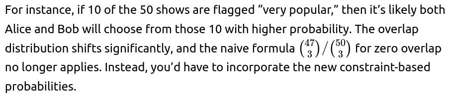
Q3: How do we handle the scenario where Alice’s picks and Bob’s picks are not uniformly random, but follow a known popularity distribution?
In real-world recommendation or preference systems, some shows might be more popular than others. Instead of each subset being equally likely, each show might have a different probability of being chosen by any given person. For instance, show #1 (a blockbuster) might have a 10% chance of being in someone’s top 3, while a niche show #2 might have only a 0.1% chance, and so on.

Pitfalls: • Overlooking the fact that in a non-uniform distribution, the probability of collision for a popular show is significantly higher than for a less popular show. • In practical scenarios, the assumption of independence might also be questionable (e.g., if Bob is influenced by Alice’s preferences).
Q4: If Alice’s picks become known to Bob before he chooses, how does this change the probability of overlap?
In some real-world scenarios, Bob might learn that Alice has chosen certain shows (e.g., if she posts her list online) before making his own selection. If Bob wants to maximize or minimize overlap, he can adapt his choice. Two distinct strategies:
• Bob wants to maximize overlap: He sees Alice’s 3 chosen shows. If Bob’s goal is to match as many as possible, he will simply pick the same 3 shows, leading to guaranteed 3 common shows. Probability of overlap is then 1 if we consider that scenario. • Bob wants to minimize overlap: If he wants to ensure zero common shows, he can avoid all of Alice’s 3 picks. He can choose from the remaining 47. In that case, the probability of no overlap is 1.
In normal question statements, we assume Bob picks blindly and uniformly. But if Bob has prior knowledge and an objective that influences his picks, the unconditional probability calculations no longer hold. The entire distribution for Bob’s selection changes because he is no longer choosing independently or randomly.
Pitfalls: • Not recognizing that knowledge of Alice’s choice makes Bob’s choice no longer independent. • Failing to reevaluate the sample space once Bob’s strategy changes.
Q5: What if they pick their top 3 shows sequentially with no possibility of overlap during selection?
Another variation is that once Alice chooses a show, Bob cannot pick that show at all, so effectively the system removes that show from Bob’s available pool. This might happen in certain “draft-style” picking processes (like fantasy sports drafts).
Computation: • After Alice picks 3 distinct shows, those 3 shows are off-limits for Bob, so Bob chooses his 3 from the remaining 47. • In that scenario, the probability of overlap is obviously 0, as it’s impossible for Bob to pick any of Alice’s chosen shows.
Pitfalls: • Confusing “no overlap” that emerges from a process constraint with a random outcome. Here, the event is forced by the selection mechanism, not by chance.
Q6: How does the probability of at least one overlap change if each chooses 4 or 5 shows instead of 3?
Here we focus on how the probability of at least one match grows as more picks are made out of the same pool. For a general scenario of each choosing k shows from n:

Pitfalls: • Overlooking boundary cases such as k close to n/2, where combinatorial effects become more pronounced. • Confusion if the scenario allows or disallows repeated picks of the same show.
Q7: Could the hypergeometric distribution be directly used to model the number of overlaps?
Yes. The overlap distribution here is a textbook hypergeometric scenario if we fix Alice’s set first and consider Bob’s random draw:
• We fix Alice’s 3 picks as a chosen subset of size 3 in a population of size 50. • Bob draws 3 items (without replacement) from the same 50. • The number of items in common with Alice’s set of 3 is the hypergeometric random variable.
In a standard hypergeometric setting, if we label the 3 items chosen by Alice as the “marked” items in a population of 50, then Bob’s draw is from that 50. The probability that X (the number of “marked” items Bob draws) takes a particular value x is:

Q8: In practical scenarios, how might repeated trials or season-based changes affect the probabilities?
In a real media-consumption environment, preferences can shift over time (e.g., new seasons or new shows become available, or user taste changes). If we measure the probability that two viewers pick the same top 3 shows at different points in time:
• The base set of 50 might change from month to month. • The “top 3” might not be truly random but influenced by marketing or social media trends. • Over long periods, the effective probability of overlap can fluctuate if some shows become massively popular or if viewers’ tastes converge.

Pitfalls: • Assuming stationarity (that the probability distribution doesn’t change over time) can lead to mismatches with real user behavior. • Overlooking real correlation structures, such as friends influencing each other’s tastes.
Q9: How do we extend this to more than two people choosing their top 3 shows?
Extending beyond two people (e.g., Alice, Bob, and Charlie each choosing 3 from 50) introduces more complicated combinatorial aspects. Common questions might be:
• “What is the expected number of shows chosen by all three?” • “What is the probability that none of them share any show?”

Pitfalls: • Exponential blow-up in the number of possible ways more than two people can overlap. • Missing that you can still rely on linearity of expectation for the expected triple-overlap, but not for distribution calculations like “probability that none of them share any show.” That requires more direct counting or repeated application of combinatorial reasoning.
Q10: Could real-world constraints like preference ordering or “must-watch” disclaimers change the naive uniform random approach?
Yes. In many real systems, user picks are not pure random draws from a set. Users might: • Have to pick at least one show from a specific category (e.g., “must watch” family-friendly show). • Have a strict preference ordering, such that if their top choice is available, they always pick it, and so on.
Each of these constraints changes the selection probability distribution. If a subset of the 50 shows is forced or more likely to be included, that subset’s overlap probability goes up.
Pitfalls: • Using uniform combinatorial logic in situations where certain picks are favored or constrained. • Underestimating how “must picks” or “extremely popular picks” can greatly increase overlap probabilities.


