
ML Interview Q Series: Sum of Uniform Random Variables ≤ 1: Probability via Multidimensional Integration

Browse all the Probability Interview Questions here.
Let X_1, X_2, …, X_n be independent random variables that are uniformly distributed on (0,1). What is P(X_1 + X_2 + … + X_n ≤ 1)? Answer this question first for n=2 and n=3.
Short Compact solution
For n=2, note that each X_i has density 1 on (0,1). Then
For n=3, we have
By extending this idea, in general,
Comprehensive Explanation
Joint Density and Setup
Each X_i is uniform(0,1), so the probability density function (pdf) for each X_i is 1 if x_i is in (0,1) and 0 otherwise. Because the X_i are independent, the joint density of the entire random vector (X_1, X_2, …, X_n) is the product of the individual densities. Specifically, for 0 < x_i < 1 for all i:
f(x_1, x_2, …, x_n) = 1.
Outside that hypercube (0,1)^n, the joint density is 0.
Probability for n=2
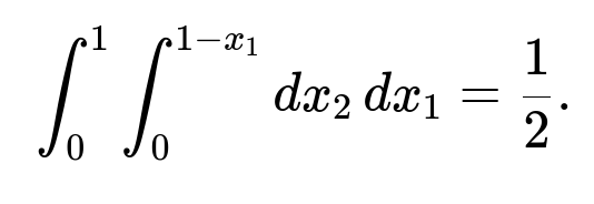
We want P(X_1 + X_2 ≤ 1). This is equivalent to integrating the joint density over the region 0 < x_1 < 1, 0 < x_2 < 1, subject to x_1 + x_2 ≤ 1. In standard text-based form, the double integral is:
integral from x_1=0 to 1 of (integral from x_2=0 to 1 - x_1) of 1 dx_2) dx_1.
This region is the triangle in the unit square where x_1 + x_2 ≤ 1. Its area is 1/2. Hence:
P(X_1 + X_2 ≤ 1) = 1/2.
Probability for n=3
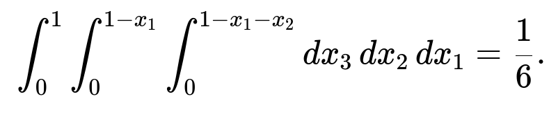
We want P(X_1 + X_2 + X_3 ≤ 1). We must integrate the joint density over the 3D region 0 < x_1 < 1, 0 < x_2 < 1, 0 < x_3 < 1, with x_1 + x_2 + x_3 ≤ 1. The region is a tetrahedron inside the unit cube. The triple integral is:
integral from x_1=0 to 1 of ( integral from x_2=0 to 1 - x_1 of ( integral from x_3=0 to 1 - x_1 - x_2 of 1 dx_3 ) dx_2 ) dx_1.
Evaluating yields 1/6.
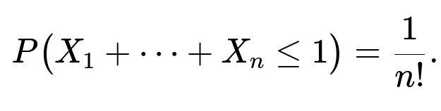
General n-Dimensional Case
In n dimensions, the region defined by x_1 + x_2 + … + x_n ≤ 1 with 0 < x_i < 1 is known to be an n-dimensional simplex (specifically, a standard simplex scaled by 1 along each axis, fitting inside the unit hypercube). The volume of that simplex is 1/n!. Because the joint density is 1 on (0,1)^n, the integral over this simplex gives:
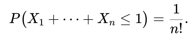
This result can be seen either by evaluating an n-fold integral inductively or by invoking the known geometric volume of an n-simplex.
Further Follow-up Questions
Why does the integration approach mirror the geometric volume?
When you integrate a constant density (equal to 1) over a region in n-dimensional space, you effectively compute the n-dimensional volume of that region. Since each X_i is constrained to (0,1), we are focusing on a subset of the unit hypercube, and the subset described by x_1 + x_2 + … + x_n ≤ 1 is precisely a simplex.
Is there a combinatorial or geometric interpretation?
Yes. The condition X_1 + X_2 + … + X_n ≤ 1 with each X_i > 0 can be viewed as partitioning a segment of length 1 into n+1 parts (the n variables plus the leftover piece up to 1). Counting that in continuous space gives the volume of the corresponding simplex, and that volume is 1/n!.
Can we prove 1/n! in a more direct geometric way?
One popular argument is that the simplex x_1 + … + x_n ≤ 1, x_i ≥ 0, can be inscribed in the hypercube [0,1]^n. By symmetry, one can show there are n! such simplices that exactly fill that hypercube without overlap. Since the hypercube has volume 1, each simplex has volume 1/n!.
How would you compute this probability numerically in Python?
We could use a Monte Carlo approach:
import numpy as np

def estimate_probability(n, num_samples=10_000_000):
    X = np.random.rand(num_samples, n)
    sums = np.sum(X, axis=1)
    return np.mean(sums <= 1.0)

# Example usage:
prob_estimate = estimate_probability(3)
print(prob_estimate)
For large n, the result should approach 1/n! as num_samples grows, although factorials can get small very quickly.
How might this generalize if each X_i has a different distribution?
If each X_i were uniform(a_i, b_i), the joint density would be the product of the individual densities on the region a_i < x_i < b_i. The integration limits and region would shift accordingly. The volume analogy would not be as direct unless all intervals were the same and the variables still maintained some structured constraints. In more general cases, the probability would be found by n-dimensional integration over the region x_1 + x_2 + … + x_n ≤ some bound.
Could you extend this to the discrete case?
If X_i were discrete uniform random variables over {1, 2, …, m}, then P(X_1 + … + X_n ≤ k) would require a summation instead of an integral. The closed-form solution might not be as simple, but generating functions or combinatorial methods (counting integer partitions under constraints) could be used.
These considerations ensure you understand both the continuous and discrete analogies, as well as computational approaches.
Below are additional follow-up questions
What if the random variables are still uniform(0,1) but are no longer independent? How does that change the probability?
When the variables X_1, X_2, …, X_n are not independent (but each still individually uniform on (0,1)), we can no longer multiply their densities to get the joint density. Instead, we would need to know or estimate the joint distribution. The condition X_1 + … + X_n ≤ 1 becomes more complicated because potential correlations (or dependencies) can make some subsets of the space more or less likely.
For instance, if the X_i are positively correlated (i.e., they tend to be large or small together), the probability that their sum remains below 1 might be significantly different from the 1/n! result that applies under independence. If they are negatively correlated (one tends to be large when another is small), it might become easier to have X_1 + … + X_n ≤ 1. Without a specific correlation structure or joint pdf, there is no simple closed-form expression like 1/n!.
A key pitfall is assuming independence formulas still hold under correlation. That leads to incorrect probability estimates. In real-world settings where measurements might inherently correlate, ignoring dependence can over- or underestimate the true probability drastically.
Could the Central Limit Theorem (CLT) help approximate the probability for large n?
If X_i are i.i.d. uniform(0,1), then each X_i has mean 1/2 and variance 1/12. By the CLT, the sum S_n = X_1 + … + X_n has approximately a normal distribution with mean n/2 and variance n/12 for large n. Specifically, S_n is roughly Normal(n/2, n/12).
However, to find P(S_n ≤ 1), we would look at (1 - n/2) / sqrt(n/12) in the left tail of that normal distribution. For large n, (1 - n/2) becomes very negative (since n/2 grows much faster than 1). The probability that S_n ≤ 1 rapidly shrinks to zero. This lines up with the fact that 1/n! also shrinks quickly as n grows. But using a normal approximation for extremely small tail probabilities can be numerically unstable.
A subtlety here is that the sum cannot exceed n, so the distribution is strictly bounded in [0, n]. Although the normal approximation is unbounded, for large n it still can give a rough sense that the probability is very small once n is bigger than a handful. A pitfall is applying the normal approximation for small n or for extreme tail events without carefully verifying its accuracy.
What if we want P(X_1 + X_2 + … + X_n ≥ 1) instead?
Since X_1 + … + X_n ≥ 1 is the complement of X_1 + … + X_n ≤ 1 only if n=2 in a trivial sense. In general, for n≥2, these events are not direct complements within the unit hypercube because X_1 + … + X_n can exceed 1 but still be ≤ n. In fact:
P(X_1 + … + X_n ≥ 1) = 1 − P(X_1 + … + X_n ≤ 1) + Probability(X_1 + … + X_n > 1 but out of (0,1)^n domain).
But since X_1 + … + X_n must lie in [0, n], if each X_i ∈ (0,1), we do have:
P(X_1 + … + X_n ≥ 1) = 1 − 1/n!,
because X_1 + … + X_n is always between 0 and n for uniform(0,1) variables. The subtlety is ensuring that the domain is restricted to the unit hypercube. Within that hypercube, the probability that the sum is ≤ 1 plus the probability that the sum is > 1 must be 1. Therefore,
P(X_1 + … + X_n ≥ 1) = 1 − 1/n!.
How does floating-point precision affect the computation of 1/n! when n grows?
For large n, n! becomes an extremely large number. Therefore 1/n! can become very small. With typical double-precision floating-point numbers, once 1/n! is smaller than around 10^-308, it underflows to 0 if you compute n! directly and then invert it. This can cause numerical issues when n is large (on the order of 170+ in double precision).
A practical pitfall is that naive direct computation of factorial and then taking its reciprocal can result in 0. If you want to handle moderate to large n, you may consider using logarithms (log(n!)) to maintain precision or using specialized libraries for arbitrary-precision arithmetic. Even for moderate n (e.g., 20!), floating-point rounding must be handled carefully, or a stable approach like the Gamma function in a library that supports high precision might be required.
How does the result change if each X_i follows a Beta distribution with parameters (α, β)?
A Beta(α, β) random variable takes values in (0,1), but with a pdf different from the uniform(0,1). The joint distribution, if the X_i are i.i.d. Beta(α, β), is still the product of their individual Beta densities. The region of integration 0 < x_i < 1 subject to x_1 + … + x_n ≤ 1 is the same, but the integrand is now ∏ f_Xi(x_i) = ∏ C x_i^(α-1) (1 - x_i)^(β-1) where C is the Beta normalizing constant. Hence the probability is:
∫( over x_1+…+x_n ≤ 1 ) ∏ x_i^(α-1) (1 - x_i)^(β-1) dx_1 … dx_n.
That integral does not simplify nicely to a single factorial expression. Instead, it can be expressed in terms of the Dirichlet distribution or incomplete Beta functions in n dimensions. There could be no neat closed form except for certain special cases (e.g., α=1 or β=1 recovers uniform). Pitfalls include applying the uniform result 1/n! by mistake. The distribution shape drastically changes the probability of being in certain regions, so direct integration or advanced special functions might be needed.
What practical relevance does P(X_1 + … + X_n ≤ 1) have in real applications?
This probability arises whenever you have normalized budgets or resources in optimization problems, reliability analysis, or partitioning tasks in systems engineering. One typical scenario is allocating tasks that each take a random fraction of some total resource capacity. The condition that the sum stays within a limit ensures no overflow. A subtlety in real systems: tasks might have minimum or maximum resource constraints that differ from uniform(0,1), or correlations might exist between tasks, rendering 1/n! inapplicable. Another subtlety is that real-world distributions might not be uniform. Using the uniform-based result in such scenarios can lead to misestimation of failure probabilities.
How would the probability formula adapt if the domain were (0,a) instead of (0,1)?
If each X_i is uniform(0,a) for some a > 0, then X_i/a is uniform(0,1). We can let Y_i = X_i/a. Then Y_i are i.i.d. uniform(0,1). The condition X_1 + … + X_n ≤ 1 becomes (X_1 + … + X_n)/a ≤ 1/a, or equivalently Y_1 + … + Y_n ≤ 1/a. Since Y_1 + … + Y_n ≤ 1/a is the same as requiring the sum of Y_i to be ≤ 1/a. However, for the event to be meaningful, we need 1/a ≥ 1, or a ≤ 1, otherwise Y_1 + … + Y_n ≤ 1/a might be trivially false for large n. If a < 1, the maximum possible sum of Y_i is n*(1). But we are trying to keep Y_1 + … + Y_n ≤ 1/a. Depending on the relationship between n and 1/a, the geometry changes. You no longer have the same straightforward n-dimensional simplex contained fully in the hypercube [0,1]^n. Instead, the region might be nonexistent if n > 1/a. Careful scaling is necessary to see if that region is nonempty.
A pitfall is directly replacing 1 with a in the final formula without addressing that the sum now must be ≤ 1 in terms of the original scaling. You should transform the variables or re-derive the volume for the region 0 < x_i < a with x_1 + … + x_n ≤ 1.
What if we integrate over 0 ≤ x_i ≤ 2 instead of 0 ≤ x_i ≤ 1?
Then each X_i is uniform(0,2) with density 1/2. The joint density would be (1/2)^n inside the hypercube (0,2)^n. The region of interest for X_1 + … + X_n ≤ 1 must be contained entirely within (0,2)^n, but the scale is larger. Notice that requiring x_1 + … + x_n ≤ 1 is actually a subset within that hypercube. If n is sufficiently large, it might be quite easy to remain under 1, but actually, if each X_i can be up to 2, the region where the sum is under 1 is relatively small. One must integrate (1/2)^n over the simplex x_1 + … + x_n ≤ 1, x_i ≥ 0. In that region, x_i never exceeds 1 anyway, but they are each allowed up to 2 in principle. So the probability is
(1/2)^n * Volume(simplex of side 1 in n dimensions).
Because the volume is 1/n!, the probability is (1/2)^n * 1/n!. A subtlety is if you had asked for X_1 + … + X_n ≤ 3, for instance, you would need to check the portion of the simplex that fully fits in (0,2)^n. For sum ≤ 3, there could be partial constraints if 3 < 2n. One must carefully define the feasible region and integrate the correct joint density.
These examples highlight that scaling the uniform range drastically affects the computation, and factoring in the correct density (1/(b-a))^n if each X_i is uniform(a,b) is critical. A pitfall is forgetting to incorporate the scaled density and using an incorrect volume measure.