
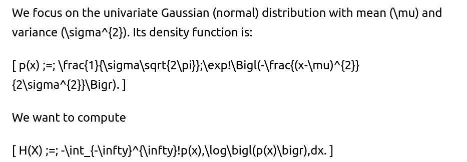
ML Interview Q Series: Suppose X is a one-dimensional Gaussian random variable with mean μ and variance σ². How can we find its differential entropy?

📚 Browse the full ML Interview series here.
Short Compact solution

Comprehensive Explanation
What is Differential Entropy?

This integral can be positive, negative, or even infinite in certain pathological cases, so it differs in several respects from discrete entropy. Nevertheless, for well-behaved distributions such as the normal (Gaussian) distribution, it gives a meaningful measure of uncertainty in terms of “nats” if we use the natural logarithm.
Gaussian Distribution Setup


This is the well-known result for the differential entropy of a univariate normal distribution.
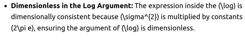
Why This Formula Makes Sense
Dependency on (\sigma): The entropy (or uncertainty) depends on (\sigma) in a logarithmic manner. As (\sigma) (i.e., the spread of the Gaussian) grows, the entropy increases.
Practical Verification via Numerics
In practice, one can numerically verify the integral definition by discretizing a normal density and approximating:
import numpy as np

def gaussian_pdf(x, mu, sigma):
    return (1.0 / (sigma * np.sqrt(2.0 * np.pi))) * np.exp(-0.5 * ((x - mu)/sigma)**2)

def differential_entropy(mu, sigma, num_points=100000, xmin=-10, xmax=10):
    xs = np.linspace(xmin, xmax, num_points)
    pxs = gaussian_pdf(xs, mu, sigma)
    # Approximate the integral -sum p(x)*log(p(x))*dx
    dx = (xmax - xmin) / (num_points - 1)
    entropy_approx = -np.sum(pxs * np.log(pxs + 1e-50)) * dx
    return entropy_approx

mu_val, sigma_val = 0.0, 2.0
approx_entropy = differential_entropy(mu_val, sigma_val)
analytic_entropy = 0.5 * np.log(2.0 * np.pi * np.e * sigma_val**2)
print("Numerical approximation :", approx_entropy)
print("Analytic formula        :", analytic_entropy)
This code demonstrates how to approximate the entropy by discretizing the domain and comparing it against the closed-form expression.
Follow-up Question 1
How does differential entropy differ from discrete Shannon entropy, and why can differential entropy be negative?
Differential entropy is defined for continuous distributions and involves an integral of (p(x)\log(p(x))). Discrete Shannon entropy, on the other hand, is a sum over discrete probabilities of the form (\sum p_i \log\frac{1}{p_i}). In discrete entropy, the value is always nonnegative (and can be infinite if any probability goes to zero).
However, differential entropy can take negative values or even be infinite, because the density (p(x)) can become very large in small intervals without violating the integral constraint. Essentially, in continuous domains, a probability density can concentrate sharply, leading to large negative contributions to (\log(p(x))). This difference highlights that differential entropy is not a straightforward generalization of discrete entropy; it does not have the same intuitive interpretation as “bits of information” that discrete entropy does.
Follow-up Question 2
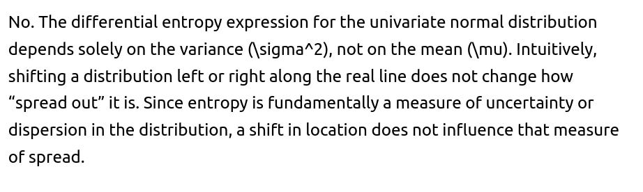
Does the location parameter μ affect the differential entropy?

Follow-up Question 3
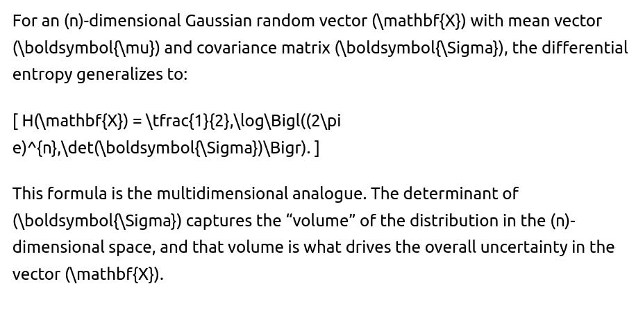
Can you extend this result to the multivariate Gaussian case?

Follow-up Question 4
What if σ² approaches 0?

Follow-up Question 5
Why do we often say “differential entropy” rather than just “entropy” for continuous distributions?
The term “differential entropy” emphasizes the fundamental difference between the continuous case and the discrete case. Unlike discrete entropy, differential entropy can take on negative values, depends on the coordinate system, and lacks certain properties that discrete entropy holds (e.g., it is not invariant under continuous transformations of the variable). By specifying “differential,” we clarify that we are dealing with the continuous version of the concept of entropy.


Below are additional follow-up questions
If we use a different logarithm base (e.g., log base 2) to define the entropy, what changes in the final expression?
When dealing with continuous distributions, we often use the natural logarithm for convenience, which yields differential entropy in “nats.” If instead you use log base 2, you get units of “bits.”

Conceptually, the shape and scale of the distribution don’t change, only the measurement unit (from “nats” to “bits”). This applies for any continuous distribution, not just the Gaussian. The only difference is a constant scaling factor.
How does differential entropy relate to Kullback–Leibler divergence for the Gaussian case?
The Kullback–Leibler (KL) divergence is a measure of how one distribution diverges from another reference distribution. In the Gaussian case, for two normal distributions with different means and variances, the KL divergence has a known closed-form solution.
Differential entropy, by contrast, is a property of a single distribution—roughly how “spread out” or “uncertain” it is in the continuous sense. KL divergence involves comparing two densities, say ( p(x) ) and ( q(x) ), via

Why can’t we directly interpret differential entropy in bits for a physical system unless we specify a reference measure?
In discrete entropy, measuring in bits is straightforward because each outcome’s probability is dimensionless and the summation is also dimensionless, so “bits” meaningfully interpret “how many binary questions” are needed to identify an outcome.
For continuous distributions, there is an added subtlety: the density (p(x)) is measured in units of “1/(value of x).” Consequently, differential entropy depends on the units of (x). For instance, if (x) is measured in centimeters vs. meters, it shifts the numerical value of differential entropy by (\log(100)).
Hence, unless we fix a specific reference measure or a certain system of units, the notion of “bits” for differential entropy can be ambiguous. This is one reason “differential entropy” can take negative values and is not as straightforwardly “the number of bits of information” as in the discrete case.
If the Gaussian is truncated (e.g., a normal distribution defined only on (x>0) and renormalized), how does that affect the differential entropy?
When a normal distribution is truncated and then properly normalized so that it becomes a valid probability distribution on a subinterval (for instance, ([0, \infty))), the differential entropy formula changes significantly.
Renormalized density: The density is no longer simply the standard Gaussian formula. It has an additional normalization factor because we exclude a portion of the real line.
Logarithm of that truncated density: When we compute (\log\bigl(p(x)\bigr)), it will now include a term (\log!\bigl(\tfrac{1}{\Phi\bigl(\tfrac{\mu}{\sigma}\bigr)})) (for one-sided truncation, for example), where (\Phi) is the cumulative distribution function for the standard normal.
Numerical integration often needed: The resulting integral for differential entropy no longer simplifies in a neat closed form, so we frequently resort to numerical methods to evaluate it.
Intuitively, truncation reduces uncertainty (since the domain is restricted), so the entropy of a truncated normal is less than that of the unbounded normal with the same variance.
If we apply a linear transformation (Y = aX + b), how does the differential entropy of (Y) relate to that of (X)?
For continuous random variables, if ( Y = aX + b ) with ( a \neq 0), there is a known relationship for differential entropy:
[ H(Y) = H(X) + \log|a|. ]
Here’s why:
Shifting by (b) does not affect differential entropy, similar to how the mean parameter (\mu) does not affect the entropy for a normal distribution.
Scaling by (|a|) contributes an additive term of (\log|a|). This arises from the Jacobian factor in the change of variables formula for probability densities.

How do we estimate differential entropy of a Gaussian distribution in real-world data scenarios, and what are potential pitfalls?


How does differential entropy connect to cross-entropy and perplexity in language modeling or machine learning contexts?
In many machine learning tasks, especially language modeling, we deal with cross-entropy as a training objective. Cross-entropy between two continuous distributions (p) and (q) is:

How do we find the differential entropy of a mixture of Gaussians (GMM) and what are potential challenges?
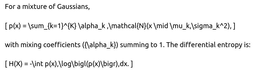
There is no closed-form solution in general for a mixture. You typically use numerical methods (e.g., Monte Carlo integration) or sophisticated approximation techniques (like bounding the log-sum-exp).
Challenges and pitfalls include:
High-dimensional integrals: For multivariate mixtures, direct integration can be extremely difficult.
Large K: Mixtures with many components can significantly complicate the computation.
Approximation errors: Approximations might be biased or have high variance unless carefully managed.
Estimation from data: If the GMM parameters are themselves only estimated from limited data, the resulting entropy estimate compounds that estimation error.
How does the concept of entropy for continuous distributions apply when the domain is inherently bounded in real-life measurements (e.g., sensor measurements that cannot exceed certain physical limits)?
Real-world sensor data often have physical limits (a device can record values only in a certain range). Strictly speaking, the underlying distribution might be effectively “truncated,” or it might be a continuous distribution with extremely steep tails near the bounds.
Implications:
If you assume an unbounded Gaussian in modeling but data are truly bounded, there is a mismatch that can affect how you interpret or compute differential entropy.
If the measurement device saturates, the actual density near the bounds might be heavily distorted relative to an ideal Gaussian.
Overlooking such constraints can lead to incorrect assumptions regarding entropy.
In such contexts, a properly truncated or bounded model can produce a more meaningful measure of uncertainty.
Suppose the data are not truly Gaussian but we assume a Gaussian for entropy calculations. What are the consequences and potential justifications?
Consequences of assumption:
The differential entropy we calculate might not match reality, because the distribution might have heavier tails (like a Student’s t-distribution) or be skewed.
If we force-fit a Gaussian, we could underestimate or overestimate the spread of the data, leading to an incorrect entropy measure.
Potential justifications:
Central Limit Theorem (CLT): If the data are aggregated from many independent factors, the distribution might be “close enough” to Gaussian in practice.
Simplicity: Gaussian models are mathematically convenient (closed-form formula for differential entropy) and often used as a first approximation.
Computational efficiency: Estimating a full nonparametric density or more complex parametric density can be expensive, while fitting a Gaussian is straightforward (only need mean and variance).
When the real distribution deviates significantly, it is prudent to check the quality of the Gaussian approximation and consider more robust estimates of the density if accuracy is essential.


