
ML Interview Q Series: Survival Probability in a Lake: A Normal Distribution Approach to Depth Risk.

Browse all the Probability Interview Questions here.
Suppose there is a 5.8-foot-tall man who cannot swim, and he intends to swim in a lake whose depth is normally distributed with a mean of 5.6 feet and a standard deviation of 1 foot. If he will drown whenever the water level exceeds his height, what is his chance of survival?
Comprehensive Explanation
A common way to tackle this scenario is to treat the lake depth as a normally distributed random variable. Let X represent the lake depth. The assumption given is that X follows a Normal distribution with mean (mu) = 5.6 feet and standard deviation (sigma) = 1 foot. The man’s height is 5.8 feet. To survive, the lake depth must not exceed his height. In probabilistic terms, we need:
Probability of survival = P(X <= 5.8).
In a normal distribution, we often convert (X - mu) to a standardized variable Z that follows a standard normal distribution (mean 0, standard deviation 1). The relationship is shown as follows.
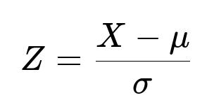
Where:
X is the random variable representing the lake depth.
mu is the mean of the distribution (5.6 feet).
sigma is the standard deviation (1 foot).
For X = 5.8, we get: Z = (5.8 - 5.6) / 1 = 0.2.
Next, we look up (or compute) the cumulative distribution function (CDF) for the standard normal at Z = 0.2. This value is approximately 0.5793. Hence:
P(X <= 5.8) = P(Z <= 0.2) ≈ 0.58.
Therefore, the probability of survival (the probability that the lake depth does not exceed 5.8 feet) is about 58%.
Below is a short Python snippet using scipy.stats.norm.cdf to illustrate how one might compute this:
import math
from scipy.stats import norm

mu = 5.6
sigma = 1.0
threshold = 5.8

# Probability that depth <= 5.8
survival_prob = norm.cdf((threshold - mu) / sigma)
print("Probability of survival:", survival_prob)
This would yield a value close to 0.58.
Potential Follow-Up Questions
How realistic is it to assume the lake depth follows a normal distribution?
Real-world lake depth distributions can be more complicated. Depth might vary across different locations in a way that is not symmetric (e.g., some parts might be very shallow, others might drop off sharply). In many cases, the depth distribution might be better represented by other statistical models or might require domain knowledge about the lake’s topography.
Why do we use the normal distribution, and what if the depth is not normally distributed?
Using a normal distribution is often a simplifying assumption. It is mathematically convenient and well-understood. However, if the actual lake depths deviate significantly from a normal shape—e.g., if the distribution is skewed or has heavy tails—then the probability estimate would be inaccurate. In practice, one might collect empirical data on lake depths and perform goodness-of-fit tests to find the best distribution.
Could the man survive in water slightly deeper than 5.8 feet if he stands on his toes or uses minor buoyancy?
The question’s premise is that he “cannot swim” and thus any depth beyond his height is lethal. In real-life situations, people might keep afloat even in water slightly deeper than their height. However, this scenario simplifies survival to a strict cutoff at 5.8 feet.
What other factors might influence survival beyond just height and depth?
Water current, temperature, and the man’s ability to hold onto nearby objects (like a boat or a ledge) could all affect survival. The question’s focus, however, is strictly on the probabilistic interpretation of depth relative to height.
Would confidence intervals for the mean and standard deviation of the lake depth matter?
If the numbers 5.6 feet (mean) and 1 foot (standard deviation) come from an estimate (e.g., from a survey of measured depths), there is uncertainty in those estimates. In practice, one might consider a confidence interval around the mean and standard deviation, leading to a range of possible survival probabilities rather than a single point estimate. This could be important if only a few samples are used to determine the average depth.
Is there a scenario where the standard deviation might be misleading?
If the lake has multiple distinct regions—some very deep, others very shallow—the overall distribution might be bimodal or multimodal rather than unimodal (single-peaked). A single standard deviation might not fully capture the spread in a multimodal distribution. Hence, the normal approximation might give a very misleading survival probability.
These considerations reflect real-life complexities that interviewers often want to see a candidate address. The key takeaway for the question is the use of normal distribution properties and standardization to compute the survival probability.
Below are additional follow-up questions
Suppose the man’s height might vary slightly instead of being exactly 5.8 feet. How would that affect the survival probability calculation?
In many real scenarios, a person’s effective height in the water can fluctuate. For instance, posture, shoe thickness, or even slight measurement errors can make someone’s actual height vary around 5.8 feet. One way to handle this is to introduce another random variable H for the man’s height. Then survival is P(X <= H) rather than P(X <= 5.8). If X is normally distributed with mean 5.6 and standard deviation 1, and H is also random (for instance, H is normally distributed with mean 5.8 and a small standard deviation representing height fluctuations), the probability of survival becomes an integral over all joint outcomes of X and H where X <= H. Symbolically, this might be expressed as:
If H and X are independent, you integrate over the region of the joint density f_X,H(x, h) such that x <= h. This can be done via numerical integration or Monte Carlo methods.
A potential pitfall is incorrectly assuming independence. For example, if the man stands up straighter in shallow water, that might correlate with the measured depth or scenario in ways that break the independence assumption.
If there is a possibility that the lake depth changes over time (due to tide, flow, or external factors), how would that influence the probability estimate?
In a dynamic environment, depth is not a static random variable but rather a time-dependent process. If we assume that depth at any instant is normally distributed with the same mean and variance, we might still use the same approach but would need to account for how quickly that depth can change relative to how long the man stays in one spot. A more robust model would consider:
Stochastic processes (e.g., a time series model) describing how water depth evolves.
The probability that at some point during the swim, the depth exceeds the man’s height.
One subtlety is that the probability of survival might drop significantly if even brief spikes in depth occur. Pitfalls include ignoring autocorrelation (depth this minute depends on depth last minute) or neglecting that the man might move to shallower areas as the depth changes.
How would the survival estimate change if the man moves around the lake, which might have varying depth distributions depending on location?
If the lake is not uniform in depth but has regions of different average depths, one would need a spatial model. For a highly variable lake, the distribution of depths might be multimodal or location-specific. The survival probability would then depend on:
The path the man takes and the time he spends in each region.
A mixing of the various distributions or a conditional distribution that accounts for different lake regions.
A potential pitfall is using just one global mean and standard deviation for the entire lake, which can be misleading if large portions of the lake are significantly deeper than 5.8 feet.
Could the depth distribution be bounded or truncated in real life, and how would that impact the probability of survival?
Yes. In reality, depth cannot be negative and typically has some maximum based on the lake’s deepest point. A normal distribution is unbounded, but a physical lake depth distribution is often bounded from below by 0 and from above by a finite maximum. If a significant portion of the lake has a shallow region near 0 feet, the lower bound might skew the distribution or cause it to deviate from the normal shape. In a truncated (or bounded) setting, the probability mass shifts within the allowed range. One must either:
Use a truncated normal distribution.
Model the distribution of depths as something like a gamma or beta distribution if it fits better.
If the distribution is truncated, the actual probability of survival may be higher or lower depending on how the truncated region affects the proportion of safe shallow depths.
What if the standard deviation or mean of 5.6 feet is just an initial estimate and not accurately measured?
If the mean or standard deviation is uncertain—perhaps derived from a small sample of measurements—there is an additional layer of uncertainty. In a Bayesian setting, one might place prior distributions on the mean (mu) and standard deviation (sigma) and then compute a posterior distribution for these parameters based on observed data. The survival probability becomes an integral over these posterior parameters:
Instead of just P(X <= 5.8), it would be an expectation of that probability over all plausible (mu, sigma).
A pitfall here is ignoring parameter uncertainty and assuming a single “best guess” for mu and sigma, which can result in overconfident estimates for survival.
How do we incorporate the situation where partial drowning is possible, rather than a strict cutoff at 5.8 feet?
The original problem sets a hard cutoff: if X > 5.8, the man drowns instantly. In practice, survival might be a decreasing function of how much deeper the water is above 5.8. One could define a probability of survival that declines as (X - man_height) increases. For instance, a logistic function could be used:
Survival probability S(x) = 1 / (1 + exp(a * (x - 5.8)))
where a is a parameter controlling how quickly survival probability drops as the water gets deeper. Then the man’s overall survival is the expected value of S(x) over the distribution of X. This approach is more nuanced but also more complicated. A major pitfall is incorrectly estimating the shape of the survival curve or ignoring real-world behaviors like panic or water currents.
Could measurement error in depth affect the actual distribution used in the calculation?
If the depth measurements that led to the mean of 5.6 and standard deviation of 1 foot contain measurement noise, that noise might artificially inflate or deflate the estimated variance. In some scenarios, the “true” variance of lake depths might be smaller, but the measurement process adds extra variability. When performing risk calculations, you should distinguish between:
True environmental variability (actual fluctuations in lake depth).
Measurement noise (errors introduced by data collection tools).
Overestimating the standard deviation might lead to a more pessimistic survival probability. Underestimating it might falsely increase confidence in survival. The pitfall is failing to disentangle these two sources of variability, potentially leading to misguided decisions.
How might human error or behavior (e.g., panic, inability to stand upright) change the simple cutoff assumption?
Even if the lake depth is at or slightly below 5.8 feet, a person who cannot swim might panic, lose footing, or fail to remain upright. This introduces a behavioral or psychological dimension not captured by a normal distribution for depth. A comprehensive model would need:
A factor representing the probability of panic or loss of balance.
An interplay between depth and individual reaction.
A key pitfall is oversimplifying the binary survive/drown condition. Real drowning risk depends on multiple human and environmental factors, not just a single numeric threshold.
What if the lake depth data was collected at intervals or from certain locations only, and the man chooses a random spot to swim?
If data collection was sparse—say only from a few locations or measured at widely spaced intervals—there might be areas of the lake that are deeper (or shallower) than recorded. The distribution (mean 5.6, std 1) could be unrepresentative of the lake as a whole. Handling this requires:
A careful sampling strategy that captures the overall depth variability.
Possibly weighting the distribution if some parts of the lake are visited more frequently.
The pitfall is blindly using aggregated statistics that do not reflect local variations. The man might pick a random location that disproportionately exposes him to deeper water, lowering his survival probability compared to the naive estimate.