ML Interview Q Series: Testing Birth Sex Ratio Hypothesis via Binomial Normal Approximation.

Browse all the Probability Interview Questions here.

Question

Suppose that of 1,000,000 live births in Paris over some period, 508,000 are boys. Suppose X is Bin(10^6, 0.5) and calculate approximately P(X ≥ 508,000). Does it seem reasonable to you that the proportion of males among Parisian babies conceived soon after the above period will be 50%? (Laplace developed his limit theorem in the late 1700’s to deal with a question similar to this.)

Short Compact solution

From a related question, one finds that the difference 508,000 − 500,000 = 8,000 corresponds to 8,000 / 500 = 16 standard deviations, because the standard deviation of Bin(10^6, 0.5) is 500. From standard normal tables, 1 − Φ(16) is on the order of 6.4×10^−58. This shows it is extraordinarily unlikely to see 508,000 or more boys if p = 0.5 truly held. Therefore, modeling births at that time and place with a p = 0.5 chance of each sex seems unreasonable. Standard practice would be to say the proportion is within a small distance of 0.508 (i.e. 508,000 / 10^6).

Comprehensive Explanation

The core idea is to interpret the number of boys out of 1,000,000 births, X, as a random variable following a Binomial distribution with parameters n = 10^6 and p = 0.5. Under a binomial model, the mean of X is np = 500,000, and the variance is np(1−p) = 250,000, so the standard deviation is 500.

The observed value is 508,000. The difference from the mean is 8,000, which is 8,000/500 = 16 standard deviations away from the expected mean if p = 0.5. This is an enormous deviation in terms of standard deviation units, making the probability of such an outcome extremely small. More formally, by the normal approximation to the binomial (Central Limit Theorem), we approximate:

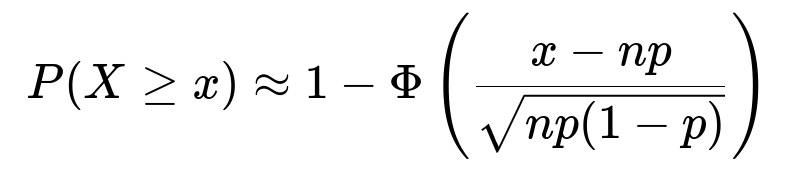
Here, X is the binomial random variable, x is the observed count of boys, n is 10^6, p is 0.5, and Φ is the cumulative distribution function (CDF) of the standard normal distribution. Plugging x = 508,000, n = 10^6, p = 0.5 gives us a Z-value = (508,000 − 500,000) / 500 = 16. Consulting standard normal tables, 1 − Φ(16) is on the order of 10^−58, indicating it is virtually impossible under an assumption of p = 0.5.

Given this incredibly small probability, it is considered implausible that the true underlying proportion p is exactly 0.5 for that historical time and location. One might suspect that the true proportion p could be slightly larger than 0.5, or that some other factors contributed to an unusual number of male births.

However, in real-world demographic studies, the proportion of male births can hover around 51% (or 0.51). Observing 50.8% might still be within a plausible range if one’s model acknowledges that historical data might not perfectly align with modern assumptions. Nonetheless, if one took the strict assumption of p = 0.5, the data would be extraordinarily unlikely.

Follow-Up Question 1: How do we use a continuity correction factor for binomial distributions, and would it matter here?

A continuity correction factor is often used when approximating a discrete distribution (like the binomial) by a continuous one (like the normal). Instead of computing P(X ≥ 508,000) by approximating it directly, one might consider P(X ≥ 507,999.5) for a more accurate normal approximation. This typically has a minor effect for very large n, and in this case—because 16 standard deviations is already so large—it does not significantly affect the conclusion that the probability is effectively zero. For more moderate deviations, a continuity correction can yield a slightly improved approximation.

Follow-Up Question 2: Could there be biological or environmental factors influencing the birth proportion?

Yes, real-world demographic data often shows a slight tilt toward male births. Factors can include maternal health, socio-economic conditions, genetics, and possibly climate or other environmental influences. Hence, the assumption p = 0.5 might be oversimplified. A more appropriate model might allow for p slightly above 0.5 (e.g., 0.51 or 0.52) to capture the biological realities of human birth.

Follow-Up Question 3: Is the Central Limit Theorem the only way to approximate P(X ≥ 508,000)?

The Central Limit Theorem is a straightforward and common approach, but for tail probabilities far from the mean—especially at 16 standard deviations—the normal approximation can become less accurate. In practice, one might rely on exact binomial calculations or use refined approximations like large deviation bounds (Chernoff bounds). However, for large n, the normal approximation tends to be quite decent. In any case, whether one uses exact methods or advanced approximations, the extremely tiny probability remains consistent.

Follow-Up Question 4: What if we want to test the hypothesis p = 0.5 using a p-value approach?

We could conduct a hypothesis test:

Null hypothesis (H0): p = 0.5. Alternative hypothesis (H1): p > 0.5 or p ≠ 0.5.

Under H0, the binomial distribution applies. We can compute the p-value as P(X ≥ 508,000). Since this turns out to be around 10^−58, we would reject H0. Such a p-value is effectively zero, confirming that the chance of observing at least 508,000 boys under the assumption p = 0.5 is astronomically small.

Follow-Up Question 5: Are there real-life datasets where a 16 standard deviation deviation might actually happen?

It is extraordinarily rare in large sample sizes for any distribution to deviate 16 standard deviations from its mean if the distribution is correctly specified. Even financial markets—known for “fat tail” events—would consider 16 standard deviations an extreme black-swan event. In typical demographic or industrial processes, seeing anything above 5 or 6 standard deviations is already astonishing. Hence, an observed 16-standard-deviation shift usually indicates the assumed distributional model might be incorrect or incomplete.

Follow-Up Question 6: How can we incorporate this kind of reasoning in machine learning or data science tasks?

In machine learning and data science, when we model certain variables with distributions (for example, a Bernoulli variable with probability p), we sometimes observe large deviations from an initial hypothesis about p. Such large deviations strongly suggest our model is misspecified. This logic is important in monitoring data pipelines or production systems: if key metrics deviate by many standard deviations from what the model predicts, it’s a signal to investigate changes in data quality, underlying population shifts, or other unseen effects.