
ML Interview Q Series: The cost function's shape (convex vs. non-convex) affects optimization. Provide an example where non-convexity helps.


📚 Browse the full ML Interview series here.
Hint: Deep neural networks are non-convex but can learn very complex relationships.
Comprehensive Explanation
Convex cost functions have a single global minimum, which means methods like gradient descent can theoretically find that global minimum. Non-convex cost functions, on the other hand, have multiple local minima, saddle points, and potentially flat regions. In practice, non-convexity may lead to challenges in optimization because an algorithm could become stuck in local minima or plateaus. Yet, non-convex functions can offer richer representational power, as they allow for modeling highly complex data distributions.
In many machine learning scenarios, convex functions are preferred for theoretical guarantees of global optimality and ease of analysis. However, modern deep neural networks typically rely on non-convex cost surfaces. This non-convexity is not just a nuisance but can be beneficial. The highly flexible parameterization of deep architectures can capture very complex and expressive representations of data, leading to superior performance in tasks like image recognition, natural language processing, and reinforcement learning.
Below is a generic form of a cost function that is commonly used in supervised learning settings:
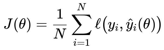
where:
N is the number of training examples.
y_i is the true label for the i-th training example.
hat{y}_i(theta) is the model's prediction for the i-th training example, which depends on the parameters theta.
ell(...) is a loss function (for instance, mean squared error or cross-entropy).
When this cost function is convex in theta, gradient-based optimization methods can reliably converge to the global optimum. But for neural networks, the function ell(...) involves complex non-linear transformations of the inputs, and the resulting cost surface in terms of theta is non-convex. Despite this, in practice, using techniques such as stochastic gradient descent with momentum or Adam often finds sufficiently good minima that generalize effectively.
Why Non-Convexity Can Be Beneficial
Deep neural networks rely on multiple layers of transformations and non-linear activations. This architecture yields a hypothesis class rich enough to approximate complex relationships in the data. While convex models (like linear regression or kernel methods with convex loss) are easier to optimize, they might not be able to capture highly non-linear relationships unless enhanced with appropriate feature engineering. Deep networks delegate this feature engineering to hidden layers, effectively “learning” features that facilitate the task at hand. This automatically learned feature extraction is a significant advantage over purely convex models, even though it introduces non-convexity into the optimization landscape.
Common Techniques to Handle Non-Convex Optimization
Gradient Descent Variants: Practitioners often use gradient descent with momentum or adaptive learning rate methods (e.g., Adam or RMSProp) to help navigate the complex, non-convex cost surface.
Initialization Strategies: Good initializations can help the parameters converge to desirable minima or at least help avoid extremely poor local minima.
Regularization: Techniques such as weight decay or dropout can smooth the optimization surface by reducing the complexity of the model, improving generalization, and sometimes aiding convergence.
Batch Normalization: Normalizing intermediate activations can stabilize gradients and can make the cost surface smoother or at least more manageable.
Example Python Code: Simple Neural Network with Non-Convex Cost
import torch
import torch.nn as nn
import torch.optim as optim

# Dummy dataset: input_size=2, output_size=1
X = torch.randn(100, 2)
y = (X[:, 0] * 2 + X[:, 1] * 3 + torch.randn(100)).unsqueeze(1)

# Simple feedforward network (non-convex cost surface)
model = nn.Sequential(
    nn.Linear(2, 10),
    nn.ReLU(),
    nn.Linear(10, 1)
)

loss_fn = nn.MSELoss()
optimizer = optim.Adam(model.parameters(), lr=0.01)

for epoch in range(1000):
    optimizer.zero_grad()
    predictions = model(X)
    loss = loss_fn(predictions, y)
    loss.backward()
    optimizer.step()

print("Final loss:", loss.item())
This neural network exhibits a non-convex cost surface due to the ReLU non-linearity and the multi-layer architecture. Despite non-convexity, in practice it usually converges to a solution that can fit the data reasonably well.
Potential Follow-up Questions
How can one distinguish between a convex and a non-convex cost function by examining the mathematical form?
To determine if a cost function is convex, observe whether any line segment drawn between two points in parameter space lies entirely above or on the surface defined by the function. Formally, a function f(theta) is convex if for all theta1 and theta2 and for all alpha in [0,1]:
f(alpha*theta1 + (1 - alpha)theta2) <= alphaf(theta1) + (1 - alpha)*f(theta2).
For non-convex functions, there exist some pairs of theta1 and theta2 for which this inequality does not hold. Practically, if your model architecture includes non-linearities like activation functions (ReLU, sigmoid, tanh) combined with multiple layers, you get non-convex cost surfaces.
Does non-convexity always result in poor local minima?
Not necessarily. In high-dimensional spaces (like deep networks), many local minima often result in comparable performance. While the optimization landscape is filled with saddle points and local minima, empirical evidence shows that many of these minima generalize relatively well. Also, advanced initialization and regularization techniques help steer the parameters toward regions that avoid pathological solutions and exhibit good generalization.
How does overparameterization in deep learning relate to non-convexity?
Overparameterized networks (having more trainable parameters than strictly needed) can navigate complex non-convex surfaces more flexibly. This large parameter space often contains numerous low-loss regions, which makes optimization easier in practice. The model can often settle in wide, flat minima that tend to generalize well.
Can methods like gradient descent theoretically get stuck in saddle points or local minima for non-convex functions?
In principle, yes. However, in high-dimensional parameter spaces, saddle points are more prevalent than deep, narrow local minima. Methods like stochastic gradient descent with momentum often help escape saddle points by adding noise and altering the effective dynamics of the optimization. Thus, while it is theoretically possible to get stuck, in practice, especially with large-scale data and networks, it tends not to be a major barrier.
What role does regularization play in non-convex settings?
Regularization techniques, such as L2 weight decay or dropout, can alter the geometry of the cost surface. By penalizing large parameter values or randomly disabling neurons, these methods can prevent the network from settling into sharp minima. Sharp minima often correspond to overfitting, whereas flatter minima tend to produce better generalization. Consequently, regularization can improve both optimization stability and generalization performance in non-convex problems.
Below are additional follow-up questions
How do different gradient-based optimization techniques handle non-convex cost surfaces differently?
Different optimization algorithms can traverse the non-convex landscape in subtly distinct ways. Stochastic Gradient Descent (SGD) often uses small random batches to approximate gradients, which can introduce noise that helps escape saddle points or shallow local minima. Momentum-based methods accumulate gradients over multiple iterations, effectively smoothing out abrupt changes in parameter updates and potentially navigating through ravines or narrow valleys more efficiently. Adam and RMSProp adapt per-parameter learning rates, mitigating issues that arise from varying gradient magnitudes across layers, and can sometimes accelerate convergence in deep architectures. However, adaptive optimizers may overfit quickly if their hyperparameters are not carefully tuned. The key idea is that each method shapes the training trajectory differently in non-convex spaces, which can either facilitate or hinder convergence depending on the model architecture, dataset size, and presence of noise. A potential pitfall is that in certain non-convex settings, more sophisticated optimizers might converge faster initially but generalize worse than plain SGD, largely because of how quickly they reduce the training loss and possibly overfit.
Why are convergence guarantees weaker for non-convex optimization, and how is this managed in practice?
For convex cost surfaces, strong theoretical guarantees ensure that gradient-based methods will find the global minimum (assuming a suitable learning rate and convergence criteria). In contrast, non-convex cost functions can have multiple local minima, saddle points, and flat regions, making it impossible to guarantee convergence to a global minimum. In practice, researchers rely on empirical results, careful hyperparameter tuning, and architectural heuristics to achieve good solutions. Common strategies include picking initialization schemes that avoid pathological regions of the parameter space, using robust optimizers with momentum or adaptive learning rates to steer the search away from sharp minima, and employing regularization techniques to simplify the landscape. One subtle edge case is small or highly noisy datasets, where non-convex models might overfit quickly and get stuck in poor regions of the parameter space, necessitating stronger regularization or early stopping.
In which real-world scenarios might we still prefer convex models over non-convex ones despite potentially lower representational power?
Convex models can be easier to interpret and analyze, making them desirable in applications such as finance or healthcare, where transparency is critical for trust and regulatory reasons. Convex models also offer more predictable optimization behavior, with no need to rely on random restarts or intricate learning rate schedules. For smaller datasets or simpler tasks, linear or convex kernel-based models might perform adequately without the risk of getting trapped in poor local minima. A possible pitfall is that relying on convex approaches in highly complex domains (such as large-scale natural language processing or computer vision tasks) can lead to underfitting unless supplemented with sophisticated feature engineering or kernel tricks. When real-time or on-device inferencing demands smaller model footprints and quicker training, convex models may also be preferred for their simplicity and lesser computational overhead.
Are there specialized optimization techniques specifically designed for non-convex cost surfaces, and how do they differ from standard gradient-based methods?
Some specialized methods, like Simulated Annealing or Genetic Algorithms, work by introducing randomness and search heuristics that can jump out of local minima. Others, like Basin-hopping, systematically explore the parameter space by searching locally and then globally attempting to find better basins of attraction. These techniques differ from standard gradient-based approaches in that they do not strictly follow gradient information at every step; they often intentionally sample from the parameter space in ways that allow them to escape difficult regions. Although this can improve the chance of finding better minima, these methods are typically slower and less scalable for high-dimensional deep learning tasks. A common pitfall is that as dimensionality grows, global search methods can become computationally infeasible, so researchers often resort to hybrid techniques (e.g., combining gradient-based optimization with occasional random restarts) rather than purely non-gradient methods.
How do skip connections or residual connections in neural network architectures affect the shape of the cost function surface?
Skip or residual connections, as used in ResNets, effectively introduce shortcut paths for gradients, which can reduce the severity of the vanishing gradient problem. These extra pathways often lead to a smoother optimization surface by allowing gradients to flow more directly through the network, thus helping to avoid certain pathological configurations. In practice, adding these connections can flatten out the cost surface or at least make it easier for gradient-based methods to traverse deep networks. A subtle edge case is that while skip connections can help with optimization, they might also enable the network to memorize noise or uninformative patterns in small datasets if regularization is insufficient, which could degrade the model’s ability to generalize.
Do advanced second-order methods, like Newton’s method or quasi-Newton methods, help in non-convex settings, and are they feasible for large-scale problems?
Second-order methods use curvature information (the Hessian matrix or approximations thereof) to guide parameter updates. In non-convex problems, the Hessian matrix can have both positive and negative eigenvalues, indicating potential saddle points. While second-order methods can potentially converge in fewer iterations because they exploit curvature, they are often too memory-intensive and computationally expensive in large-scale deep learning. Quasi-Newton methods can approximate second-order information with less computational overhead than exact Hessian computations, but they can still be challenging for very high-dimensional parameter spaces. A pitfall is that naive implementations of second-order methods might easily get stuck at saddle points in non-convex spaces where the Hessian does not provide a straightforward direction of steepest curvature descent. Thus, such methods are rarely used in mainstream deep learning and instead see niche use where the dimensionality is more manageable or where a precise solution is paramount.
Could model interpretability or debugging become more complicated when dealing with non-convex cost surfaces?
Non-convex neural networks often have millions or billions of parameters, making it very difficult to understand how each parameter influences the final decision boundary. Interpreting why the optimization algorithm converged to a specific local solution can be nearly impossible because of the complex, high-dimensional error surface. Debugging training issues—such as exploding or vanishing gradients—can also be more challenging because these problems might not have straightforward solutions in non-convex frameworks. In contrast, convex models like linear or logistic regression provide direct coefficients that can be interpreted, at least in principle, as feature importance. However, advanced interpretability methods (e.g., saliency maps or Shapley value-based methods) attempt to address these concerns for deep networks. One subtlety is that these interpretability techniques themselves rely on assumptions about gradients or local perturbations, which might fail to capture global behaviors or interactions between parameters in a non-convex landscape.
How do we decide if we have found a “good enough” local minimum, and when should we invest in further hyperparameter searches?
In practice, one often monitors validation loss, training loss, and occasionally additional metrics like accuracy or F1 score. If the model’s validation performance stagnates or begins to degrade due to overfitting, it may indicate that further fine-tuning of hyperparameters (learning rate, regularization factors, or model architecture) is necessary. Alternatively, if validation performance plateaus for multiple restarts or multiple seeds, it is possible that the model has reached a region of the parameter space where improvements are unlikely without increasing capacity or collecting more data. A pitfall is prematurely concluding that a local minimum is optimal. Sometimes, changing just one hyperparameter—like switching to a different optimizer or altering the learning rate schedule—can significantly improve performance in a non-convex setting. Another subtlety is that performance can fluctuate significantly in the early epochs, so robust early stopping criteria and repeated trials are often essential.
Can the shape of the loss landscape affect how quickly a model converges or how stable training is from run to run?
Large flat regions or plateaus can slow down training, causing gradient-based optimizers to make only minimal progress until they find a slope to descend. Steep ravines can cause erratic gradients, leading to significant parameter jumps and unstable learning. Additionally, random initialization can position the model at varying starting points in the high-dimensional space, causing run-to-run variability in outcomes. Some architectures or activation functions are more prone to these issues. For instance, certain activation functions without careful initialization might produce widespread dead neurons (e.g., ReLU units stuck at zero). Good initialization, careful selection of optimizer hyperparameters, and normalization strategies such as batch normalization often reduce this variability. Edge cases appear when the dataset is highly imbalanced or extremely noisy, as the gradient signals can be misleading, exacerbating training instability across runs.
Does the shape of the cost function surface change how we approach distributed training or hardware acceleration?
When parallelizing large models across multiple GPUs or across distributed systems, different mini-batches might be processed on different nodes, potentially causing asynchronous updates to the parameters. Non-convex surfaces can amplify this challenge, as inconsistent parameter states can make it harder for the network to settle into a stable region of the cost surface. Techniques such as synchronous updates, gradient averaging, or gradient compression can mitigate these issues but introduce communication overhead or latency. Another subtlety is that certain hardware accelerators or mixed-precision training approaches can introduce numerical instabilities (e.g., float16 overflow) that can hinder convergence in steep or chaotic regions of the non-convex surface. To address this, frameworks include methods like loss scaling and specialized numerical routines to preserve precision.