
ML Interview Q Series: Time Series Validation: Correctly Evaluating Models Using Walk-Forward Splits.
📚 Browse the full ML Interview series here.
Time Series Model Validation: For a time-series forecasting model, why is randomly shuffling data for cross-validation a bad idea? Explain how you would correctly evaluate a model on time-series data (for example, using a rolling forecast origin or hold-out the last segment of time for testing). Describe a time-based split or walk-forward validation approach that respects the temporal order of data to avoid lookahead bias.
Understanding Why Random Shuffling is Problematic for Time-Series When dealing with time-series forecasting, the crucial element is the temporal order of observations. The target variable at a given time often depends on earlier points in time. If you shuffle data randomly, you discard the time-based structure and can inadvertently allow the model to learn from “future” data points when predicting past observations. This leads to lookahead bias and yields overoptimistic estimates of model performance. In real deployments, the model will only have access to past data when generating future predictions, so training and evaluation must respect the chronological order.
Core Concept of Lookahead Bias Lookahead bias arises if, during either training or validation, information from a future time step is indirectly fed into the model for predicting earlier steps. For example, if you randomly shuffle your dataset, then data from time t+1 could appear in the training set while you are trying to validate predictions at time t. This would not reflect real-world performance at all. Hence, the entire principle of time-series validation demands that no sample from the future can be included in the training set when predicting the past or present.
Proper Method for Time-Series Model Validation A common best practice is to keep the sequence in correct time order and split such that the model is first trained on an initial segment of data up to a certain time, then tested or validated on the next segment. This ensures that each point you test on is strictly in the “future” of what the model has already seen. Typical approaches include:
Holding Out the Most Recent Data A straightforward strategy is to split off the most recent time period (e.g., last few days, months, or years) as a test set, and train the model on all data preceding that. You do this because in a real deployment, you want to predict the future. Hence you hold out the actual future portion of data for final validation. This method preserves temporal ordering.
Rolling (or Walk-Forward) Forecast Origin Instead of a single training/validation split, a more robust approach uses multiple splits. For instance, you can set an initial training window, train the model up to a certain date, then test on the next time slice, then roll forward by expanding or moving the training window to include new data, and then test on a subsequent slice, and so forth. This approach simulates multiple points in time at which you re-train or update your model. It also gives a series of out-of-sample error estimates, showing how your model evolves over time and handles different market conditions, seasonal changes, or distribution shifts.
Sub-Sampling Windows Another variant is to use multiple sliding windows of training data. For each window, train on data from time t to time t+k, then evaluate from time t+k+1 to t+k+m. You then slide forward by some step size. This technique can be repeated across the entire timeline so that you get multiple validation metrics, each corresponding to different periods. The final metric can be averaged to measure the overall forecast performance while preserving time order in all splits.
How to Implement Time-Based Splits (High-Level Code Illustration) Below is an illustrative example in Python pseudocode using scikit-learn or a similar library. The crucial part is that the splitting is done in chronological order, not by random selection.
import numpy as np
import pandas as pd
from sklearn.model_selection import TimeSeriesSplit
from sklearn.linear_model import LinearRegression

# Suppose data is sorted by time, oldest -> newest
df = pd.DataFrame(...)  # Some time-series dataset
X = df.drop('target', axis=1).values
y = df['target'].values

# TimeSeriesSplit example
tscv = TimeSeriesSplit(n_splits=5)  # number of splits

for train_index, test_index in tscv.split(X):
    X_train, X_test = X[train_index], X[test_index]
    y_train, y_test = y[train_index], y[test_index]

    model = LinearRegression()
    model.fit(X_train, y_train)
    predictions = model.predict(X_test)
    # Evaluate error metrics, e.g. MSE or MAPE on y_test
In a production-grade time-series forecasting scenario, you would also pay close attention to stationarity, possible seasonal structure, the presence of exogenous features, and data transformations that might be required to make the forecasting approach more robust. Nonetheless, the essential aspect is never to shuffle data in a way that breaks chronological order.
Walk-Forward Validation Mechanics in Detail When performing a walk-forward approach:
You define an initial training set that spans from the beginning of your data up to a specific time. You fit the model on this data and then forecast over a short horizon immediately after the training window. You record the forecast accuracy using an appropriate metric. You then “walk forward” in time by adding the newly observed data to the training set. You refit the model (depending on whether you do an expanding window or fixed window) and then forecast the following period. This procedure continues until you reach the end of your dataset, yielding multiple estimates of the forecast performance across different time segments.
The main advantage is that you get a realistic assessment of how your model would perform in a real-time setting where data arrives sequentially. You also capture changes in distribution over time. The main drawback can be higher computational cost, because you’re fitting a model multiple times.
Mitigating Distribution Shifts and Non-Stationary Phenomena Time-series often evolve over time. The data distribution in an early interval may not match the data distribution in a later interval. Proper time-series validation is essential for revealing whether a model can handle shifting patterns. If you were to shuffle data randomly, you might incorrectly average over the entire timeline, ignoring subtle drifts and changes in the process generating the data. Using time-based splits and analyzing performance in successive segments provides better clarity on how well your model adapts to shifts.
Potential Metrics for Forecast Evaluation Common metrics include Mean Squared Error (MSE), Mean Absolute Error (MAE), or Mean Absolute Percentage Error (MAPE). One might define MAPE as:
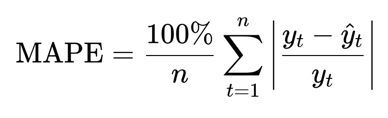
where ( y_t ) is the actual value at time t and ( \hat{y}_t ) is the predicted value at time t. It measures the percentage error relative to actual demand or actual outcomes.
Validating Over Different Forecast Horizons A single-step forecast predicts only the next time point (e.g., next day). A multi-step forecast might predict the next several steps (e.g., next 30 days). In each scenario, you must structure your training/validation so that the horizon you evaluate is consistent with what you will do in production. A time-based split remains crucial for avoiding any contamination of the training set by future samples.
Edge Cases and Possible Pitfalls One subtlety occurs if you have external regressors or exogenous variables. You have to ensure that those features also do not leak future information. For example, if you have a variable that is only available with some delay in real life (like the next day’s weather forecast only available on the previous day), you must replicate that delay carefully in your training data setup. Otherwise, you could inadvertently give the model “future” exogenous variables that would never be available in real-time prediction.
Another potential pitfall is that certain time-series do not only depend on local history but also on cyclical or seasonal patterns. One should verify that the chosen splitting approach is capturing seasonality. If you have strongly seasonal data (e.g., daily retail data with strong weekly patterns), you might ensure that each training window is at least multiple seasonal cycles long so that the model has a chance to learn those patterns.
Data frequency also matters. In high-frequency trading data (e.g., tick-by-tick data in finance), the time-based split might be on a much shorter horizon, and the number of walk-forward slices might be quite large. The data can also have abrupt shifts due to market conditions. Proper walk-forward validation helps you see how quickly or slowly your forecasting model adapts to those changes.
Follow-Up Question: How does walk-forward validation differ when using an expanding window versus a sliding (or rolling) window?
When performing time-series validation, you can manage the training set in two main ways: an expanding window approach or a sliding window approach.
Expanding window approach means that for each new validation period, you add (append) new data to the training set while still retaining all the old data. Over time, your training set becomes larger. This approach assumes that older data remains relevant for predicting the future. It is often used for processes where you believe that historical patterns remain valuable indefinitely, or you want the model to absorb the maximum amount of data available.
A sliding (or rolling) window approach means you keep the window size fixed (or somewhat bounded) and move it forward in time. In each iteration, you discard the oldest portion of the data and incorporate the newest data. This is useful for processes suspected to have evolving or drifting distributions, where older data might no longer represent current dynamics. You want your model to be trained on the most relevant recent history.
The difference mainly revolves around how big the training set is at each step, and whether or not you consider the entire past data to remain relevant to the future. The choice depends on domain knowledge (e.g., whether the process is strongly drifting or if older data remains informative).
Follow-Up Question: Why is preserving temporal order important for avoiding lookahead bias, and can you explain a real-world example?
Preserving temporal order is crucial because data in future time steps must not influence the model’s parameters or hyperparameters when predicting earlier (or concurrent) time steps. In forecasting, the entire point is to predict what has not happened yet. If the validation procedure allows future data to creep into the training phase, you end up with predictions that implicitly rely on information that would never be available in real-world deployment. This artificially inflates performance metrics and can result in models that fail when truly deployed.
As a simple real-world example, imagine you have daily sales data for a store, and you are trying to predict tomorrow’s sales. If you randomly shuffle your dataset, you might have rows from next week’s sales data in your training set while validating on last week’s data. That will produce a misleadingly low error metric because the model “knows” next week’s demand patterns, which is impossible in a real scenario. By preserving the time order, you only train on historical data and test on data that actually comes after the training data in time, which reflects the real forecasting scenario.
Follow-Up Question: How would you decide the length of the training window in walk-forward validation?
Choosing an appropriate training window length is often domain-specific. Generally, you look at:
The stationarity or seasonality of the data. If there are strong seasonal effects (weekly, yearly, etc.), your training window should be at least as large as the longest seasonal cycle so the model can capture these patterns. Data availability and volume. If you have a lot of data, you may keep a larger window, but if data is scarce, you might be forced to use all historical points. Possibility of concept drift. If the underlying distribution shifts over time, a smaller, more recent window might yield more accurate forecasts for the upcoming period at the cost of ignoring older patterns that might be less relevant. Computational constraints. Fitting large models repeatedly can be time-consuming, so you might limit the size of the window to reduce computational overhead.
In practice, it can be beneficial to experiment with different window lengths and measure out-of-sample performance to find the best trade-off between capturing historical patterns and focusing on recent trends.
Follow-Up Question: How do you handle hyperparameter tuning in time-series models without leaking future information?
When tuning hyperparameters for time-series forecasting, it’s essential to ensure your tuning procedure also does not use any future data to pick hyperparameters. This is sometimes called nested cross-validation for time-series:
You can implement a time-series cross-validation approach, where for each fold, you split the data into training and validation segments that respect time. Within the training portion of each fold, you further split that training data (also respecting chronological order) to tune the hyperparameters. You select the best hyperparameters based on performance on the validation portion within that fold, and then you evaluate on the outer fold’s test set. You repeat this for each fold and average the performance metrics.
This procedure ensures that your hyperparameter choices remain free of future data information. If you don’t do this, you risk picking hyperparameters that are overfitted to future test sets.
Follow-Up Question: Could you illustrate an approach for dealing with multiple seasonalities or exogenous features in a walk-forward time-series context?
In real-world scenarios such as retail forecasting or energy load forecasting, you often have multiple seasonalities (daily, weekly, yearly) plus exogenous inputs like weather data, promotions, events, etc. In that situation:
You incorporate those exogenous features (e.g., daily temperature, holiday indicators) into your feature matrix at each time step, ensuring that for each forecast horizon you only use exogenous data that would realistically be available at prediction time. For instance, if you know next-day’s weather forecast is updated each evening, you only feed that forecast into the model once it is actually published. You maintain the same walk-forward or time-based splitting logic. For each fold, you train on a chronological slice of data that includes both your target and exogenous features up to time t, then you validate on times t+1 to t+m. Because multiple seasonalities might exist, you may need a sufficiently large training window for your model to observe at least one full cycle of each seasonality. Or you might incorporate frequency-based transformations (like Fourier series or dummy variables for seasonality) into your feature engineering. By using multiple expanding or rolling splits, you examine how your model’s performance changes under different seasonal regimes or over different times of the year.
Follow-Up Question: Why might a simple hold-out method not be enough for certain time-series models?
A single hold-out method (training on an earlier block of time and testing on the final block) can be a good preliminary check. However, it does not confirm whether the model is stable across different time intervals. If you only have one train/test split, you might get a single performance estimate that is not representative of all market conditions or environmental variations that occur in the data’s history. Many time-series can have periods of anomaly or unique events (e.g., sudden economic shocks, pandemics, extreme weather, or holiday surges). A single hold-out might train on data that doesn’t properly represent those anomalies or might test on a region with unusual events that the training set never saw.
Multiple rolling splits or walk-forward validation solves this by creating multiple train/test partitions, each corresponding to a different forecast origin. You get a series of performance metrics across time, which can be more robust for determining how your model might perform in various scenarios. This is especially relevant in FANG-level challenges, where data can be non-stationary and unpredictable.
Follow-Up Question: Are there any alternative methods to walk-forward validation if the dataset is extremely large?
Yes. If the dataset is extremely large (e.g., decades of high-frequency data), repeatedly retraining your model on the entire historical dataset for each fold can be computationally expensive. Some strategies include:
Using a fixed-width rolling window to limit the size of training data. Incremental or online learning techniques in which your model updates its parameters with new data in a more efficient manner rather than retraining from scratch. Sampling strategies that maintain time continuity but skip certain intervals to reduce training complexity. For example, training on a shorter, more recent block and only occasionally including older intervals if they are relevant for capturing rare events.
These methods help reduce computational costs while still preserving chronological order. However, each approach must be carefully validated to make sure you still avoid lookahead bias.
Follow-Up Question: How do you decide the number of rolling splits for walk-forward validation?
Choosing the number of splits (n_splits) in a TimeSeriesSplit or similar approach is typically a trade-off between:
Having enough splits to thoroughly evaluate performance in different time segments. Ensuring each training set is of reasonable size and that each test set is large enough to produce reliable error metrics. Avoiding excessive computation.
If you have a long time horizon, you might create many splits, each focusing on a short forecast window. If your forecast horizon is relatively short compared to your entire dataset, you can afford more splits. Conversely, if you have fewer data points or long seasonal cycles, you may have fewer splits so that each training set covers the essential seasonal patterns. Ultimately, the choice is governed by domain knowledge, data size, seasonal/holiday patterns, and computational constraints.
Follow-Up Question: Could you illustrate how to measure performance across multiple splits in a walk-forward evaluation?
Yes. When you do multiple splits, after each training/validation step, you compute a metric such as MAE, MSE, RMSE, or MAPE. Let’s say you denote each split’s error as ( e_i ) for the i-th split. You can aggregate them in simple ways:
You can average those errors:
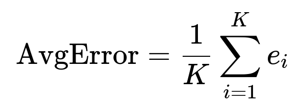
You can also look at the median or percentile of errors if outliers are a concern. This way, you see an aggregated performance measure. More advanced methods can involve weighting splits differently if some intervals are more critical. In practice, the average or median error across splits is a straightforward measure of overall forecast performance.
Follow-Up Question: How does the correct evaluation strategy tie in with model deployment and maintenance in a real system?
After you have validated your model in a time-series-consistent way, you often deploy it to generate forecasts in production. Because time-series data is continuously generated, you might implement a schedule (for instance, daily or weekly) to retrain or update the model with the newest data. This is effectively the walk-forward approach but done online:
At each new step (e.g., each day), you take all available historical data, retrain or update the model, then produce the forecasts for the upcoming horizon. You keep track of forecast performance as the real data arrives and can feed that performance information back into your pipeline to decide whether your model is degrading over time (concept drift). If the model degrades, you might investigate whether you need a new architecture, additional features, or a different hyperparameter configuration.
Thus, your entire pipeline, from training to validation to final deployment, respects the time order and ensures no future data is used at any point.
Below are additional follow-up questions
How do you handle missing data or irregular time steps in walk-forward validation?
Missing data or irregular time gaps can disrupt the continuity of your time-series and complicate the creation of training/validation segments. If observations at certain time steps are absent, you risk an inaccurate view of the temporal relationships. A practical way to address this is:
Identify the Nature of the Missingness Determine if the data is missing at random, missing completely at random, or if there is a systematic cause (for example, sensors failing during specific times). If missingness is not random, you need to investigate the cause because it might hint at underlying processes that should be modeled separately.
Impute or Transform For time-series data, a common approach is forward filling or backward filling to maintain continuity. However, you must ensure that the method chosen does not leak future values. Forward fill uses the last known value to fill missing points, which is typically safe as it does not require future data. Alternatively, you can interpolate between observed points if the data is expected to change smoothly.
Resampling If your data is at irregular intervals, you can resample to a fixed frequency (e.g., daily, hourly) and fill in missing timestamps. This ensures that each time step is accounted for, even if originally it was missing. This also allows easy slicing of intervals for rolling splits.
Dedicated Methods for Irregular Time Series Some forecasting frameworks are built to handle irregular time steps directly, especially in fields like survival analysis or event-based processes. In such cases, you preserve the data in its raw form but carefully implement the walk-forward splits so each split still respects the chronological order of events.
Check Impact on Validation Missing data or irregular steps can cause large uncertainties during your validation phase. For instance, if many consecutive days are missing, your training set or test set might be artificially compressed. The best practice is to keep track of how much data you drop or impute and to measure whether it alters the distribution or patterns the model sees.
Can you discuss strategies for aligning external (exogenous) data that come in different frequencies or with delays in time-series forecasting?
Time-series forecasts often rely on exogenous variables such as weather data, economic indicators, or user behavior metrics. These exogenous series might have a different sampling frequency or become available with a delay. In a real deployment scenario, you cannot use a data point about tomorrow’s exogenous variable if it will only be published tomorrow afternoon. Strategies include:
Temporal Alignment Establish a clear timeline for each exogenous feature. If your main series is daily, aggregate or resample external data to daily frequency. If the external data is available at an hourly level, you can compute daily averages, daily max/min, or other relevant transformations.
Lagging or Shifting Features If the exogenous data is known only after a certain lag (e.g., an economic indicator that publishes with a one-month delay), you might shift that feature so that the value that belongs to time t is only fed to the model at t+1 or whenever it becomes available. This ensures no leakage of future knowledge.
Handling Different Frequencies If your main series is monthly but exogenous variables are available daily, you can roll them up (e.g., average daily temperature over the month). Alternatively, if your main series is at a higher frequency but exogenous data is monthly, you can propagate that monthly value to every day within the month. Always be explicit about how you handle boundary conditions—especially if monthly data is published mid-month rather than at the start.
Walk-Forward Splitting with External Data When splitting the dataset, ensure that both your target and exogenous features are aligned so that any row in your training or test set only contains exogenous variables that realistically would have been known at that time. If you do repeated expansions or sliding windows, replicate this alignment for each window.
What steps do you take if the data generation process itself changes over time, potentially invalidating older segments of the time-series?
In real-life applications, processes can drift or even undergo abrupt regime changes (e.g., policy changes, technology upgrades, new product launches). If older data becomes less predictive:
Segment the Timeline Identify the period before and after the change. One might train separate models for each regime or disregard data that is too old if it no longer contributes to future trends. However, it is often important to keep some historical context if the events might recur.
Recalibration Windows Use a smaller rolling window that focuses on the most recent data. This helps the model adapt more quickly to new patterns rather than being swayed by outdated historical behavior.
Change-Point Detection Implement algorithms that detect changes in distribution, so you can systematically re-train the model or switch to a new model when the process shifts. This might involve monitoring metrics like average error or drifting distribution statistics.
Contextual Features You can add binary or categorical features that indicate which regime the data belongs to. This allows a single model to learn different patterns for different regimes, although it only works if these regimes repeat or if the transitions hold stable properties.
How can you adapt walk-forward validation to handle real-time streaming data in production environments?
In continuous data environments (e.g., streaming sensor data, live transactions), the forecasting process must dynamically update:
Online Training or Incremental Learning Rather than re-fitting a batch model from scratch every time a new data point arrives, use algorithms that update parameters incrementally. Libraries like River (formerly known as Creme) in Python support incremental learning for time-series.
Micro-Batching If fully streaming updates are not feasible, you can set small time intervals (e.g., every hour or day) to retrain the model on the latest data. Each retraining event is a smaller-scale version of walk-forward, effectively shifting the window forward by a small step.
Rolling Evaluation Window Continuously keep track of forecast accuracy in a rolling window. For instance, once new data arrives for time t+1, compare it to your forecast from t. This real-time error monitoring helps detect concept drift or breakpoints in the underlying process.
Latency and Resource Constraints In streaming scenarios, you might have strict latency requirements. Some complex models (like large neural networks) can be expensive to retrain frequently. You may need an approach that strikes a balance between accuracy and retraining speed (e.g., partial retraining, or layer freezing in deep networks).
What should you do if your time-series dataset is extremely short or extremely long?
Extremely Short Time-Series If you have fewer data points, you face challenges like limited context for capturing seasonality or trends and insufficient data for multiple splits. Potential solutions include:
Collect Additional Data: If feasible, gather more historical data from archives or combine multiple related but non-identical series (transfer learning or domain adaptation).
Simple Models First: Start with simpler statistical models (e.g., ARIMA) that are less prone to overfitting. A large neural network might not be suitable for very limited data.
Single Train/Test Split: If you truly have just a short sequence, you may only do a straightforward hold-out approach to get a rough estimate of performance. Validation is tough, so interpret the results carefully.
Extremely Long Time-Series If you have massive data (such as decades of daily or intraday data):
Use a Rolling Window: Keep a subset of the most relevant data, or else model training can become unwieldy.
Parallelize or Use Efficient Libraries: If you do repeated walk-forward splits, it might be computationally heavy. Consider distributed computing frameworks or approximate training methods.
Summarize or Segment: If the data is unwieldy, you can segment by year, month, or context. Then do a hierarchical approach, first analyzing each segment, then unifying or ensembling the results.
If your forecast horizon changes over time, how do you maintain a consistent walk-forward validation?
Sometimes you need to forecast 1 day ahead in one scenario and 7 days ahead in another scenario. You might shift the forecast horizon depending on user needs or business requirements:
Separate Models or Multi-Horizon Models You can maintain separate models for each forecast horizon or use multi-horizon models (like seq2seq or transformers-based approaches) that predict multiple future steps at once. For walk-forward splits, each split must include data for training and evaluation that matches each horizon of interest.
Staggered Walk-Forward For example, if you want to predict at horizons of 1, 3, and 7 days, for each training/validation period, you forecast all three horizons. Then you measure performance on each horizon separately. This approach ensures that your validation addresses each horizon’s predictive performance.
Realistic Data Availability Ensure that for a 7-day horizon, you only use exogenous inputs that would be known at the time of the forecast. This is more complicated than single-step forecasting, so keep track of which features are available for which forecast lead time.
How do you measure the statistical significance of forecast improvements when using time-based splits?
When comparing two or more forecasting models, you want to know if the performance difference is real or just noise:
Diebold-Mariano Test A commonly used statistical test for forecast accuracy comparison. It compares forecast errors from two models over a certain time horizon. The test can account for autocorrelation in the forecast errors, which is crucial in time-series.
Paired T-Tests with Block Bootstrapping Traditional paired t-tests assume independent samples, which is not always true in time-series. A block bootstrap approach resamples contiguous blocks of residuals to preserve temporal dependencies.
Rolling Window Performance Another way is to gather forecast errors from each time-based split, treat them as repeated trials, and apply standard statistical tests with caution. You might consider that each time-based split is an independent scenario. If you have enough splits, you can compute averages and confidence intervals.
How do you handle abrupt, one-time future events (like a sudden lockdown or unplanned outage) that the model has never seen in historical data?
Unprecedented events can break even the best time-series forecasts:
Scenario Analysis One approach is scenario-based modeling, where you hypothesize the possible impact of an event. If a lockdown or outage is truly unprecedented, your model can’t infer from historical patterns. You might artificially create or simulate data that reflects changes in consumer behavior or system usage under lockdown.
Expert Overlays In many industries, a domain expert might override or adjust the statistical model’s prediction for special events. For instance, they might add or subtract a certain magnitude based on experience.
Anomaly or Intervention Models Models like intervention analysis (e.g., in an ARIMA framework) can handle known structural breaks. However, if the break is wholly new, you might detect it after the fact and switch to a new model or add a special feature to flag post-event data.
Could you discuss how to handle potential target leakage that might arise from derived features in time-series?
Sometimes features are derived from the same target you are trying to predict, inadvertently introducing leakage:
Proper Lagging of Derived Features If you compute a rolling average or rolling sum of the target variable, ensure that your rolling window only uses data up to time t-1 to predict time t. If you use the sum from t+1 to t+5 while predicting t, that’s immediate leakage.
Purging Future Observations In a walk-forward or rolling split, ensure that any feature that references future data is purged or delayed. For example, if you have an indicator for “the maximum price in the next 24 hours,” that is obviously not known at the current time step in a real scenario.
Cross-Validation with Proper Feature Engineering All feature engineering that depends on future data must be done after you partition your dataset so that each training set does not contain any future knowledge. If you do the feature engineering on the entire dataset first and then split, you risk subtle leakage.
What if your time-series is highly non-stationary and includes multiple structural breaks—how do you ensure your walk-forward validation is robust?
In some domains (e.g., finance, user engagement for a rapidly growing platform), the time-series might break stationarity often:
Multiple Rolling Splits with Short Windows A shorter rolling window can adapt to quickly changing patterns. This ensures that older data that no longer represents current behavior does not skew model training.
Diagnostic Tests Perform stationarity tests (like Augmented Dickey-Fuller) on different segments of your data. Identify large changes in mean, variance, or autocorrelation structure. If certain segments are extremely different, a single global model might be insufficient.
Model Specialization You might build different models specialized for different regimes (e.g., normal conditions vs. peak load conditions). For each walk-forward step, detect the current regime, then pick or train the appropriate specialized model.
Adaptive Approaches Use methods that can internally adjust to changing distributions, such as recurrent neural networks with dynamic state, or advanced models that incorporate a notion of drifting weights. But always maintain a time-based validation approach to confirm the model’s ability to adapt to these shifts.
How do you address class imbalance or rare events in time-series forecasting when the target is not continuous but categorical or event-based?
Sometimes forecasting deals with classification or event detection (e.g., “Will an extreme weather event happen tomorrow?”). If events are rare:
Focal Loss or Weighted Loss When training, apply appropriate loss functions that give higher weight to the minority class. However, keep your time-based split intact. This ensures your model sees chronological examples of rare events only when they happened.
Synthetic Oversampling Techniques like SMOTE can be tricky for time-series because they randomly interpolate between minority class samples, potentially violating time-order. If used, it must be done only within each training window, never mixing data from future time steps.
Evaluation Metrics Accuracy can be misleading if the event is rare. Use metrics like precision, recall, F1, or area under the precision-recall curve (AUPRC). For time-series, ensure you measure these metrics in a rolling test set scenario to confirm real-world performance.
Feature Engineering for Leading Indicators In many real-time scenarios, you want advanced warning of a rare event. Incorporate known leading indicators if available. Make sure those indicators are realistically available prior to the event in your walk-forward validation.
What are common pitfalls when applying deep neural networks for time-series forecasting under a rolling/expanding validation scheme?
Deep learning offers flexibility and power for time-series but can introduce unique pitfalls:
Long Training Times Deep nets can take substantial time to train. Re-training a large architecture multiple times in walk-forward splits can be expensive. You might need to do partial re-training or freeze certain layers.
Overfitting to Non-Stationary Data Neural networks can memorize patterns in older data that are no longer relevant. With time-based splits, you might discover that performance deteriorates on the final splits if distribution has drifted substantially. Regularization, dropout, or data augmentation can help mitigate overfitting.
Data Normalization Normalization (e.g., mean-variance scaling) can be a source of data leakage if you compute global means and variances from the entire dataset before splitting. Instead, compute and apply normalization statistics from the training set only, then apply them to the test set. In a rolling scheme, recalculate or update normalization statistics each time you move the window.
Lack of Interpretability Deep models can be black boxes, making it hard to diagnose forecast failures. Thorough evaluation in multiple splits over different time segments is critical. You might also incorporate interpretability approaches (e.g., integrated gradients) but must do so within each time segment to see how the model’s interpretation changes over time.
How do you handle operational constraints like maximum model training time or memory limits during repeated time-based validations?
Industrial or large-scale forecasting systems can face constraints in compute resources:
Sampling or Subsetting Instead of training on all historical data for each fold, you might use a subset (e.g., the most recent year) if that portion is the most relevant to future predictions.
Incremental Updates Some models can be updated incrementally, bypassing the need to retrain from zero each time. This reduces overall computational load.
Parallelization Time-based splits can be run in parallel if you have enough compute resources, because each split is an independent training/validation cycle.
Caching Intermediate Results You can cache feature engineering outputs or partially trained models. For instance, if your model architecture supports partial re-training, reuse the parameters from the previous fold as the initialization for the next fold. Make sure any caching does not cause data leakage across folds.
How do you ensure your walk-forward validation remains fair if you continually tweak the model or features between splits based on prior test results?
It is easy to repeatedly look at results from each fold and adjust your approach, effectively incorporating knowledge from the test fold back into the model for future folds:
Proper Separation Between Development and Final Test You might treat the earlier folds as “development folds,” adjusting hyperparameters and features based on that feedback. Then keep the final fold (representing the most recent data) as a purely held-out test set you do not touch until you lock down your model.
Nested Time-Series CV In a more formal approach, for each outer fold, you do an inner time-series CV for hyperparameter tuning. The outer test fold is only used for final evaluation. That way, the final test performance remains unbiased by repeated model tweaking.
Careful Logging and Governance In practical teams, it is crucial to version your data, code, and model configurations. If you keep adjusting the model based on each new test set, it essentially becomes part of your training data. Maintain a strictly separate final test period that you only check once you are truly ready to evaluate.
How do you approach model selection when you have multiple candidate models using a rolling/expanding window validation?
When you have an ensemble of candidate models (ARIMA, XGBoost, LSTM, etc.):
Aggregate Error Across Splits Compute average error metrics for each candidate across all splits. Whichever model has the best overall performance is typically selected.
Consider Stability Sometimes a model might have an excellent average performance but large variance across splits, indicating potential instability. Another model might have a slightly worse average but more stable performance. Depending on your risk tolerance, you might prefer the more stable model.
Statistical Tests Use tests like Diebold-Mariano or others that compare errors from each model across each split to see if the differences are statistically significant.
Ensemble Approaches If multiple models capture different aspects of the time-series, you can combine them (e.g., a weighted average of forecasts). This can smooth out weaknesses of individual methods.
How do you handle the situation where the test set is very different from the training period in time-series forecasting?
Real-world data can shift drastically. If your test set distribution diverges from the training set:
Model Retraining or Adjustment Analyze the root cause of the shift. If it’s permanent (like a new technology standard), you might permanently change your model features, structure, or training data. If it’s transient, you might incorporate special indicators or event flags for that period.
Flexible or Non-Parametric Models Models like random forests or gradient boosting can sometimes adapt better if you keep retraining them regularly with new data. They do not rely as heavily on stationarity assumptions as certain classical time-series models.
Segregated Training If you expect such shifts to recur in the future, gather data from past episodes of similar nature (if they exist) and create a specialized “shift-aware” segment in your training set. For purely novel shifts, you can only adapt after the shift begins.
Could you discuss the impact of time granularity (e.g., minute data vs. daily data) on walk-forward validation?
Granularity significantly affects how you construct and interpret time-based splits:
Intraday vs. Daily In minute-level or second-level data (high-frequency data), a single day might already contain many thousands of observations. You might have frequent walk-forward steps (e.g., training on the first 4 hours of data and predicting the 5th hour). Ensure you handle the seasonality that occurs within a single day (e.g., morning vs. afternoon in finance).
Aggregation or Downsampling If you have extremely granular data, you might consider aggregating to a coarser resolution to reduce noise and computational load, especially if your forecast horizon is not extremely short. However, you may lose some signal that exists at high frequency.
Multiple Horizons Short-term forecasts may be more accurate if you use high-frequency data. If you plan to forecast many days ahead, minute-level data might be too noisy or might not be necessary. Decide on a granularity that aligns with your forecast horizon and business needs.
Data Volume High-frequency data can lead to massive storage and training overhead. For rolling splits, you might reduce the length of the historical window or use incremental learning to manage this.