
ML Interview Q Series: Unbiased vs. Consistent Parametric Estimators: Understanding the Key Differences.

Browse all the Probability Interview Questions here.
What does it mean for an estimator to be unbiased in parametric estimation, and how does that differ from being consistent? Provide an example of an estimator that is unbiased but not consistent, and another that is biased but consistent.
Short Compact solution
An estimator is called unbiased when its expected value equals the true parameter value. It is called consistent if, as the number of samples grows, the distribution of the estimator narrows around the true parameter.
A classic example of an unbiased but not consistent estimator is the very first sample from a normal distribution. Its expectation matches the true mean, but as the sample size increases, this single observation does not converge in its distribution to the true mean.
A well-known example of a biased yet consistent estimator is the sample variance defined by

Its expected value is not exactly the true variance due to the factor of n instead of (n−1), so it is biased. However, the bias diminishes as n increases, making it consistent for the true variance in the limit.
Comprehensive Explanation
Unbiased Estimator

However, unbiasedness alone does not guarantee other desirable properties such as low variance or good concentration around the true parameter.
Consistent Estimator

Example of Biased But Consistent Estimator
A straightforward example is the sample variance computed with a divisor of n instead of n−1:

Potential Follow-Up Question 1
What are the advantages or disadvantages of using an unbiased estimator versus a biased but consistent estimator?
An unbiased estimator has the advantage that its average “hits” the true value. However, that alone does not ensure low variance. A biased but consistent estimator might systematically under- or over-estimate in finite samples, but if it converges to the true parameter and often has smaller variance for finite sample sizes, it can be very practical. In real applications, an estimator with slightly lower bias can sometimes have much higher variance, leading to worse overall performance. Hence, there is a trade-off between bias and variance in actual estimation.
Potential Follow-Up Question 2
Can you explain the difference between convergence in probability and almost sure convergence for estimators? Is consistency the same as almost sure convergence?
Convergence in probability means that for any ϵ>0,
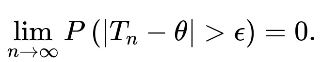
Consistency is typically defined as convergence in probability. Almost sure convergence is a stronger form of convergence which states that
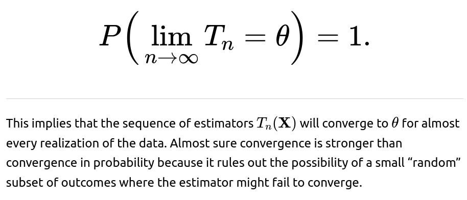
In practice, many standard estimators (like the sample mean) are consistent in both senses, but for general theoretical treatments, you must distinguish these two types of convergence.
Potential Follow-Up Question 3
Why does the sample variance with n in the denominator underestimate the variance?
When we use

Potential Follow-Up Question 4
Is an estimator that is both unbiased and consistent always preferable?
Not necessarily. In practice, you also must consider the variance, computational complexity, and other factors like robustness or whether your problem deals with heavy-tailed distributions. It is possible to have an estimator that is unbiased and consistent but has a higher variance than a slightly biased method. Depending on the application and the risk tolerance for errors, practitioners may prefer a small, stable bias over a larger variance.
Potential Follow-Up Question 5
How would you demonstrate in a simulation that the sample variance with n is biased but consistent?
You could run a Monte Carlo simulation in Python:
import numpy as np

def biased_sample_variance(data):
    return np.mean((data - np.mean(data))**2)

true_mean = 0.0
true_sigma = 2.0
n_experiments = 10_000

for sample_size in [5, 10, 50, 100, 1000, 10000]:
    estimates = []
    for _ in range(n_experiments):
        data = np.random.normal(true_mean, true_sigma, sample_size)
        var_est = biased_sample_variance(data)
        estimates.append(var_est)
    mean_est = np.mean(estimates)
    print(f"Sample size={sample_size}, Mean of variance estimates={mean_est:.4f}, True variance={true_sigma**2}")
By running this code, you will see that although the mean of the variance estimates is lower than 4.0 (the true variance) for finite samples, it approaches 4.0 as the sample size grows. This empirical observation confirms that the estimator is biased for small n but converges to the true variance as n becomes large, hence showing consistency.
Below are additional follow-up questions
When might you prefer a biased estimator that has a lower mean squared error (MSE) over an unbiased estimator?
An estimator’s MSE consists of both variance and squared bias. Even if one estimator is unbiased, it might have a higher variance than another estimator that is biased but more stable (lower variance). For many practical applications—such as real-time systems or small-sample-size scenarios—estimators that minimize overall MSE are more desirable if they reduce large fluctuations, even at the cost of some bias.
Pitfall: Overemphasizing unbiasedness can lead you to overlook an estimator’s potentially large variance. In practice, you might prefer slightly biased estimates if they yield better predictive or inferential accuracy.
Edge Case: When sample sizes are extremely large, the difference in variance between an unbiased and a slightly biased estimator might be negligible, making the unbiased approach preferable. Conversely, at small sample sizes, you often see significant variance reductions from certain biased methods.
Real-World Issue: In finance or medical decision-making, large variance can translate to higher risk. A small bias might be acceptable if it leads to more stable decisions or smaller confidence intervals.
Does the sample mean remain unbiased and consistent if the data are not independent and identically distributed?
The classic proof of the sample mean being unbiased and consistent assumes i.i.d. observations. If the data are not i.i.d., the situation becomes more nuanced:
Unbiasedness: Even if samples have differing distributions or correlations, the sample mean can still be unbiased if the expected value of each observation remains the same and if those expectations sum up in a straightforward way. However, biasedness can arise if the sampling process itself skews the mean (for instance, in certain time-series models with trends or in non-stationary processes).
Consistency: For consistency, we need some form of the Law of Large Numbers (LLN). If data points are dependent, the strong or weak LLN might not hold under the usual conditions, especially in the presence of complex autocorrelation or time trends. To ensure consistency, we typically need either a mixing condition (for weakly dependent processes) or stationarity plus suitable conditions that mimic the i.i.d. scenario.
Pitfall: Blindly assuming i.i.d. data for a time series or data with heavy autocorrelation can lead to incorrectly concluding that the sample mean converges properly. If the process is shifting or trending, your mean estimate may be systematically off.
Edge Case: In random fields or advanced time-series with long-range dependency, even stationarity might not suffice if the data exhibit heavy tails or fractal-like correlations.
How does the presence of outliers or heavy-tailed distributions affect the choice between unbiased or biased but consistent estimators?
Outliers and heavy-tailed distributions can heavily skew common estimators such as the sample mean and sample variance:
Robustness: An estimator that is unbiased for Gaussian-like data might be highly sensitive to even a single extreme outlier. Sometimes, robust estimators (e.g., trimmed means, Huber estimators) are intentionally biased but exhibit better real-world performance under heavy tails or contamination.
Pitfall: Assuming that a theoretically unbiased estimator for a normal distribution remains the best choice under heavy-tailed distributions is dangerous. You might end up with extremely high variance or unstable estimates.
Edge Case: In distributions with infinite or near-infinite variance (e.g., certain power-law distributions), even the sample mean may not converge in the usual sense. Alternative estimators (like median-based approaches) can be more reliable and stable.
Real-World Issue: Finance, insurance, and climate studies often feature heavy-tailed phenomena. A slightly biased robust method that down-weights outliers can drastically improve predictive power, even though it is not unbiased under the standard definition.
What is the difference between “strong consistency” and “weak consistency,” and how does that relate to unbiasedness?
Weak Consistency (also called convergence in probability): This is satisfied if for every ϵ>0, the probability that the estimator deviates from the true value by more than ϵ tends to zero as the sample size grows. Formally,


Relation to Unbiasedness: Neither strong nor weak consistency implies unbiasedness, and an unbiased estimator need not be strongly consistent. It is possible to have an unbiased estimator that fails to be consistent (like taking the first sample) or a biased estimator that is strongly consistent (like the sample variance with n in the denominator).
Pitfall: Students often conflate convergence in probability with being unbiased. They are distinct concepts: unbiasedness is about the expected value in finite samples, whereas consistency (in either sense) is about the long-term behavior as sample size grows.
Edge Case: For complicated data-generating mechanisms (e.g., random graphs or Markov chain models), proving almost sure convergence can require advanced probabilistic tools and might not always be feasible.
How does asymptotic efficiency tie in with unbiasedness and consistency? Can an estimator be asymptotically unbiased but still less efficient?
Asymptotic Efficiency: An estimator is said to be asymptotically efficient if, among a class of consistent estimators, it achieves the lowest possible asymptotic variance. A common reference is the Cramér-Rao bound, which sets a lower bound on the variance for an unbiased estimator. Asymptotic efficiency focuses on the estimator’s behavior for very large n.
Asymptotic Unbiasedness vs. Full Unbiasedness: An estimator that is asymptotically unbiased may have a small bias for finite n, but that bias vanishes as n grows. Even so, it can still have a larger variance than another estimator that is both asymptotically unbiased and lower in variance. Hence, the first might be less efficient.
Pitfall: Achieving asymptotic efficiency often requires strong assumptions (e.g., maximum likelihood estimators under correct model specification). If those assumptions are violated, an “inefficient” estimator might be more robust and practical.
Edge Case: In high-dimensional settings or when n is not substantially larger than the dimensionality, the entire notion of efficiency can be overshadowed by complexities such as regularization, which may introduce bias but reduce variance dramatically.
Real-World Issue: Many real-world datasets do not necessarily grow to extremely large sample sizes, or they have complicated dependencies. So, an estimator’s performance at moderate sample sizes might matter more than its limiting behavior, making “textbook” efficient methods less appealing in practice.