
ML Interview Q Series: Uncorrelated Yet Dependent Random Variables: Constructing and Understanding a Counterexample.

Browse all the Probability Interview Questions here.
Suppose we have two random variables X and Y. What does it mean for them to be independent, and what does it mean for them to be uncorrelated? Can you construct an example where X and Y are uncorrelated yet not independent?
Short Compact solution
Uncorrelatedness, on the other hand, only requires that the covariance between X and Y is zero, which translates to E[XY]−E[X] E[Y]=0.
A classic example of uncorrelated but not independent variables is where X takes values -1, 0, +1 with equal probability (1/3 each), and Y is defined to be 1 whenever X=0 and 0 otherwise. By calculation, E[X]=0, E[XY]=0, so the covariance is zero and hence X and Y are uncorrelated. However, they are not independent because if we observe that X=0, then Y is guaranteed to be 1, which is different from Y being 1 with probability 1/3 marginally.
Comprehensive Explanation
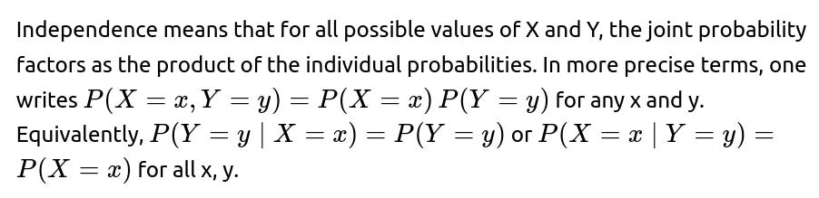
The concept of independence between two random variables X and Y is quite strong: it tells us that knowing the exact value of X gives no additional information about the distribution of Y (and vice versa). Mathematically, it is stated as P(X=x,Y=y)=P(X=x) P(Y=y) for every x and y in the support of X and Y. This definition implies that all joint probabilities factor into individual probabilities.
Uncorrelatedness, by contrast, is a weaker notion. Two random variables X and Y are uncorrelated if their covariance is zero, or equivalently if E[XY]=E[X] E[Y]. The important point is that zero covariance captures only the absence of a linear relationship, but does not capture more complex dependencies.
To illustrate how zero covariance does not guarantee independence, one can design pairs of variables whose distributions are arranged in such a way that their linear relationship (as captured by correlation) is canceled out, yet they are still very much dependent. The example in the short solution is a neat demonstration:
Let X be equally likely to be -1, 0, or +1.
Define Y to be 1 whenever X=0, and 0 otherwise.
In this case:
The expectation of X is 0, because it takes -1, 0, and 1 with equal probabilities.
The product XY is 0 in every scenario: if X is -1 or +1, then Y is 0; if X is 0, then X·Y = 0 anyway.
Hence E[XY]=0. Simultaneously, E[X]=0 and E[Y] is 1/3, so $E[X] E[Y] = 0.0... and the covariance is zero. This establishes uncorrelatedness.
However, they are not independent: if you know that X=0, you immediately know Y=1. But in the unconditional sense, Y=1 only 1/3 of the time. That difference alone is enough to show they do not satisfy the factorization property of independence.
This distinction—uncorrelated vs. independent—frequently arises in many interview contexts because it underscores a common misunderstanding: uncorrelated random variables are not guaranteed to be independent, unless one places more restrictions on the distribution (for example, if the variables are jointly Gaussian, zero correlation does imply independence, but for general distributions it does not).
How to Illustrate This Example in Practice
One might simulate these variables in Python to confirm the correlation numerically:
import numpy as np

# Large number of samples
num_samples = 10_000_000

# Generate X, taking values -1, 0, +1 with equal probability
X = np.random.choice([-1, 0, 1], size=num_samples, p=[1/3, 1/3, 1/3])

# Define Y = 1 if X=0, else 0
Y = (X == 0).astype(int)

# Compute correlation coefficient
corr = np.corrcoef(X, Y)[0, 1]
print("Estimated correlation:", corr)
We would expect the correlation (which is a normalized version of covariance) to be extremely close to zero, confirming that X and Y are uncorrelated. Yet, from the definition, if we observe X=0, then Y=1 with probability 1, proving non-independence.
Follow-up question 1: What is the difference between independence and zero correlation in a more general sense?
Independence implies zero correlation, but zero correlation does not necessarily imply independence. Independence is a complete lack of statistical dependence, whereas zero correlation only rules out linear relationships. Non-linear dependencies can still exist even when the correlation is zero.
Follow-up question 2: In what situation would zero correlation imply independence?
If two variables X and Y follow a bivariate normal (Gaussian) distribution, then zero correlation implies independence. This specific property holds for jointly Gaussian variables because their entire relationship structure is captured by their means, variances, and covariance. Outside of jointly Gaussian cases (or some other specialized families of distributions), zero correlation is not enough to conclude independence.
Follow-up question 3: How do you usually estimate correlation and independence from data?
Correlation is often estimated via sample covariance divided by the product of standard deviations. In practice, one might use Pearson’s correlation coefficient, which measures the strength of a linear relationship.
Testing independence more broadly can be done using various statistical tests:
Mutual information tests (where mutual information is zero if and only if the variables are independent).
Non-parametric methods like the distance correlation or kernel-based independence tests.
Graphical approaches (scatter plots) can help visualize non-linear relationships that a simple correlation coefficient might miss.
Follow-up question 4: Could we see a zero sample correlation in real data but still have dependence?
Yes. With enough data, a sample correlation might approximate the true correlation well. However, one can still encounter real-life examples where the true correlation is zero even though there is dependence (for example, a symmetric U-shaped relationship). In finite samples, spurious or near-zero correlations can appear. It’s always helpful to visualize your data and potentially apply more robust tests for independence.
Follow-up question 5: Are there measures other than correlation that might capture more general dependence patterns?
Yes. Correlation is essentially a measure of linear dependence. Other approaches include:
Spearman’s rank correlation, which captures monotonic relationships.
Mutual information, which captures the general notion of shared information between two random variables and is zero if and only if the variables are truly independent.
Non-linear measures like distance correlation and kernel-based measures, which can detect a broader range of dependencies.
Follow-up question 6: If X and Y are uncorrelated, does it imply their means are related somehow?
Not necessarily. Zero correlation itself doesn’t directly impose restrictions on the means other than the fact that E[XY]=E[X] E[Y]. One can have many different distributions with many different mean values and still end up with zero correlation. Correlation concerns how two variables deviate from their mean in a coordinated (linear) way. Their individual mean values might be large, small, or zero, and it doesn’t prevent them from having or not having zero correlation.
Below are additional follow-up questions
If two random variables are uncorrelated, how does that relate to the idea of orthogonality in a vector space?
Uncorrelatedness is often analogized with orthogonality because, in many linear-algebraic interpretations, covariance is a measure of how two variables "align" when considered as centered vectors. In a vector space of random variables, saying the covariance is zero loosely parallels saying two vectors are orthogonal.
However, there are potential pitfalls:
Orthogonality in a vector space is strictly about a dot product being zero. While covariance can be seen as an expectation-based dot product, the analogy doesn’t hold fully for all probability distributions, especially when moments are not well-defined or infinite.
Even with well-defined moments, zero covariance (like zero dot product) can fail to capture non-linear alignments in a probabilistic sense. Orthogonality is purely a linear notion, ignoring non-linear dependencies.
So, while the concept of orthogonality provides some intuition for uncorrelated variables (zero "projection" on each other in an expected sense), it should not be conflated with independence.
Does uncorrelatedness extend naturally to multiple variables, and how might that differ from mutual independence?
For more than two random variables, uncorrelatedness can be tested pairwise: each pair of variables must have zero covariance. One can also define a covariance matrix for a set of variables. If all off-diagonal entries in this covariance matrix are zero, we say the set of variables are mutually uncorrelated.
However, pitfalls include:
Pairwise uncorrelatedness does not guarantee mutual independence. For example, you can have three random variables X, Y, and Z where each pair is uncorrelated, but collectively they exhibit a non-linear relationship.

Hence, moving from two to many variables compounds the difference between zero covariance and full independence.
How might the finite support or discrete nature of random variables affect the detection of dependence or uncorrelatedness?
When X and Y have finite discrete support, one can theoretically compute exact probabilities for each combination of values in the support. Detecting dependence can be done precisely by checking whether P(X=x,Y=y)=P(X=x) P(Y=y) for all x, y.
But practical pitfalls arise when:
Sample sizes are small relative to the size of the support. One might not observe all possible outcomes, leading to biased or zero-frequency estimates, making it harder to accurately estimate joint probabilities (and thus covariance or independence).
Overfitting or underfitting could happen if we rely on naive empirical estimates for probabilities.
The number of parameters to estimate grows rapidly with the dimensionality of the support, which can make rigorous testing for independence computationally challenging.
In time series analysis, if two time series have zero cross-correlation at certain lags, does it imply that the series are independent?
In time series, one might compute cross-correlations at various lags to see if two signals move together over time. Zero cross-correlation at all lags often suggests no linear predictive power of one series on the other. However, the caveats include:
Zero cross-correlation at one lag does not imply zero cross-correlation at other lags. A time series can be correlated at a delayed offset.
Even if cross-correlation is zero at all lags, there might be non-linear temporal relationships, such as squared terms moving together or periodic phenomena.
Independence in time series typically requires more sophisticated tests, often involving joint distribution properties, not just correlation-based checks.
Thus, concluding independence solely from zero-lag (or even multi-lag) cross-correlations is risky if non-linear dependencies or complicated temporal patterns exist.
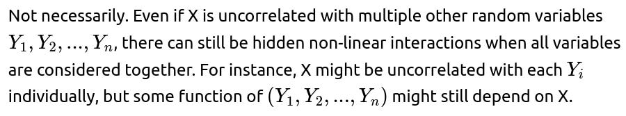
If X is uncorrelated with all components in a large set of variables, does that imply X is independent of the entire set?

Pitfalls:
The bigger the set, the more potential for complex multivariate relationships that pairwise correlations fail to capture.
The concept of conditional independence often arises in such scenarios: X might be conditionally dependent on one variable given the values of others.
What if we want to remove correlation from data? Can we "whiten" our variables, and does that ensure independence?
"Whitening" typically transforms random variables so that they become uncorrelated and all have unit variance. One standard procedure is to compute the covariance matrix, apply an eigenvalue decomposition, and use the corresponding matrix to decorrelate the variables.
Potential pitfalls:
Whitening only guarantees zero cross-covariance; it does not guarantee that the resulting components are mutually independent unless we make strong assumptions about their joint distribution (e.g., if the data are multivariate Gaussian).
For non-Gaussian data, whitening can help with some tasks (like principal component analysis), but strong non-linear dependencies might remain even after whitening.
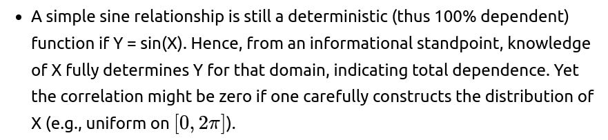
Can random variables that exhibit a strong periodic relationship be uncorrelated?
Yes, certain periodic or oscillatory patterns can lead to zero average product even when there is a clear relationship. For example, if X is uniformly distributed on an interval, and Y is a sine function of X with mean zero, the integral over one full period might end up being zero, yielding zero covariance.
However, the pitfalls in concluding independence are:

This highlights the direct and classic example: correlation does not see purely sinusoidal dependencies that are centered in a certain way.
How might missing data or censoring affect estimates of correlation or independence?
Missing data and censored observations present significant challenges:
If data is not missing completely at random, the distribution of observed pairs (X,Y) might not reflect the true underlying distribution. Hence, sample-based estimates of correlation or joint probabilities will be biased.
Techniques like multiple imputation or modeling the missing data process are required for accurate inference. But even sophisticated methods can struggle if the mechanism producing missingness is unknown or if there is heavy censoring.
Independence tests become more complicated, because one might incorrectly detect or fail to detect dependencies if a particular region of the sample space is underrepresented.
In real-world applications, data scientists must be cautious with partial data, as naive correlation or independence checks might produce misleading conclusions.
Could non-stationarity in data lead to misleading conclusions about correlation or independence?
Non-stationarity means the statistical properties of the data (like mean or variance) change over time or across different segments. This can mislead correlation estimates:
If one calculates correlation on data pooled over a changing distribution, short-term correlations might be masked or exaggerated.
Independence tests that assume a single stationary distribution might fail if the underlying process changes. One might see spurious “relationships” simply because of distribution shifts.
Analysts often split the data into segments or use time-varying parameter models to tackle non-stationarity. Failure to do so can incorrectly suggest zero correlation or false independence.
In practice, especially with economic or financial time series, non-stationarity is a critical concern that must be handled with specialized techniques before concluding anything about correlation or independence.
Does symmetry in a joint distribution automatically imply zero correlation or independence?
Symmetry alone does not guarantee either. For instance, one might have a symmetric joint distribution around (0,0), but that distribution could still have non-zero correlation or other dependencies. The distribution’s shape and how mass is concentrated matter more:
A bivariate distribution can be symmetric across the origin, yet have a strong elliptical shape that reveals a clear positive correlation.
Alternatively, one could create a symmetrical, cross-shaped distribution that yields zero correlation but exhibits high dependence in the sense that X is often non-zero when Y is near zero, and vice versa.
Hence, the presence or absence of symmetry is not a definitive indicator of correlation or independence, though it can sometimes simplify computations and inferences if one has the right symmetrical structure (e.g., elliptical symmetry in a Gaussian context).