
ML Interview Q Series: Uncorrelated X+Y and X−Y: Understanding the Equal Variance Requirement.
Browse all the Probability Interview Questions here.
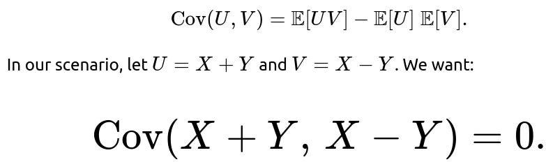
Suppose we have two random variables X and Y. Under what condition are X+Y and X−Y uncorrelated?
Under the usual definition in probability theory, two random variables are uncorrelated if their covariance is zero. So we need to analyze the covariance of X+Y and X−Y. The question is: when is

Below is an extensive explanation of the reasoning and the important details surrounding this condition, plus possible follow-up questions and answers.
Understanding the Covariance Expression
The covariance of two random variables U and V is defined as

Hence


So

Meanwhile,

Putting these together:


Hence:
Therefore, for X+Y and X−Y to be uncorrelated, we need:

Thus, X+Y and X−Y are uncorrelated precisely when X and Y have the same variance.
Intuition and Subtle Points
When random variables have equal variances, the positive “spread” contributed by X is essentially balanced by the negative “spread” from Y when we form X−Y, in such a way that the cross-term influence cancels out in the covariance calculation. Notice that the derivation did not require any assumption on Cov(X,Y) itself; that part canceled out in the algebraic expansion. Similarly, no special assumptions about means (such as zero-mean) were necessary—everything works out as long as the difference in variances is zero.
Although they are uncorrelated under this condition, remember that uncorrelated does not necessarily mean independent. If X and Y do not follow a jointly Gaussian distribution or some other specific conditions, X+Y and X−Y might still be dependent. However, from the perspective of linear correlation, the condition of equal variances in X and Y alone is enough to drive their covariance to zero.
Real-World or Practical Insights
If you ever see a real system where the sum and difference of two signals exhibit zero correlation, it is often a sign that the two signals have similar “energy” or magnitude of fluctuations. In many signal processing or communications applications, analyzing sums and differences of signals can help identify certain symmetrical properties. The condition that Var(X)=Var(Y) can also arise in scenarios where X and Y are identically distributed (though identical distribution is not strictly required if they merely share the same variance).
Below are some additional questions that a skilled interviewer might ask to probe deeper, along with thorough answers.
What if X and Y have different means? Does that affect the condition?
Even if X and Y have different means, our derivation shows that the covariance Cov(X+Y, X−Y) simplifies to Var(X)−Var(Y), completely independent of their means. The difference in means does not appear in the final condition for uncorrelatedness. So X+Y and X−Y are uncorrelated if and only if Var(X)=Var(Y), regardless of the values of E[X] and E[Y].
How would this change if we instead required X+Y and X−Y to be independent?
Uncorrelatedness is a weaker condition than independence. In general, requiring independence of X+Y and X−Y usually imposes stricter conditions on X and Y. For instance, if X and Y are jointly Gaussian random variables, then uncorrelatedness implies independence. In that special Gaussian case, the condition Var(X)=Var(Y) plus the fact that Cov(X+Y,X−Y)=0 would mean X+Y and X−Y are indeed independent. However, for arbitrary distributions, X+Y and X−Y can be uncorrelated (under the same-variance condition) but not independent unless further assumptions (such as joint Gaussianity or linear relationships) are also satisfied.
Could X+Y and X−Y be uncorrelated if either X or Y is a constant?
If one variable is a constant, say Y=c with variance 0, then Var(Y)=0 while Var(X) might be nonzero. The difference in variances will not be zero unless Var(X) is also zero (which would mean X is also constant). If both are constants, then all sums and differences are trivially constant and uncorrelated (the covariance is zero because there's no variation). But if only one is constant, they will not satisfy Var(X)=Var(Y) unless Var(X)=0 too.
Why does Cov(X,Y) vanish from the final expression?
When you expand Cov(X+Y,X−Y) in a typical scenario, you see terms like Cov(X,X), Cov(X,−Y), Cov(Y,X), and Cov(Y,−Y). Usually, you might expect cross-covariance terms to remain. But note that Cov(Y,X)=Cov(X,Y), and one appears with a plus sign, the other with a minus sign, causing them to cancel perfectly. This reveals a neat symmetry: the cross-terms do not affect the covariance in this specific combination of sum and difference. The only terms left are Var(X) and −Var(Y).
Can we verify this condition programmatically with a simple simulation in Python?
Yes, we can do a straightforward empirical simulation to verify that if X and Y have the same variance, the empirical covariance of X+Y and X−Y is near zero.
import numpy as np

# Fix a random seed for reproducibility
np.random.seed(42)

# Generate X and Y with the same variance
# For example, X ~ Normal(0, 1), Y ~ Normal(10, 1)
# so they have the same variance (1), but different means (0 vs 10)
N = 10_000_000
X = np.random.normal(0, 1, size=N)
Y = np.random.normal(10, 1, size=N)

# Form X+Y and X-Y
U = X + Y
V = X - Y

# Compute empirical covariance
cov_UV = np.cov(U, V, bias=True)[0, 1]  # Index [0,1] in the covariance matrix
print("Empirical covariance:", cov_UV)
If you run this code, you should see that the empirical covariance is extremely close to zero (the larger the sample size, the closer to zero it becomes). The difference in means does not affect this result, only the difference in variance does. If you were to change the variance of Y so that it differs from that of X, then the covariance of X+Y and X−Y would no longer be near zero.
What if X and Y have the same variance, but are correlated?
Even if there is a nonzero correlation between X and Y, the algebraic expansion shows that these cross terms cancel out in Cov(X+Y,X−Y). So the correlation between X and Y does not interfere with the result. All that matters is Var(X)=Var(Y). In effect, the sum and difference can be uncorrelated even if X and Y themselves exhibit correlation.
Could you elaborate on a practical scenario where X and Y might have equal variances but not be independent?
Consider a finance application where X and Y represent daily returns of two stocks that are typically correlated because they are in the same market. The two stocks might have distinct expected returns (means), but over the long term, the day-to-day fluctuation magnitudes (their variances) could be quite similar. Even if these two stocks have some correlation (positive or negative), if their variances match exactly, X+Y and X−Y will still have zero covariance. However, the correlation between X and Y in general remains nonzero, showing that uncorrelatedness of X+Y and X−Y does not guarantee independence.
Are there any potential pitfalls in applying this condition?
One subtlety is that uncorrelated random variables do not imply causation or independence. Also, in real datasets, the observed or estimated variances might be close to—but not exactly—the same. Numerical approximation and finite data can lead to estimates that are not exact. You might mistakenly conclude that X+Y and X−Y are uncorrelated when, in fact, you simply do not have enough data to differentiate the variances. Always check confidence intervals or run further hypothesis tests to confirm.
A second subtlety is that the condition Var(X)=Var(Y) is purely about second-order statistics. Higher moments (like skewness and kurtosis) can also create dependencies in sums and differences in more complicated ways, but the second-order measure of correlation is determined by variances and covariances only.
How can this insight be extended to more than two random variables?
In summary, how do you concisely restate the condition?
For two random variables X and Y, the sum X+Y and the difference X−Y are uncorrelated precisely when:
Var(X)=Var(Y).
No other assumptions (about means, correlation between X and Y, etc.) are needed.
Below are additional follow-up questions
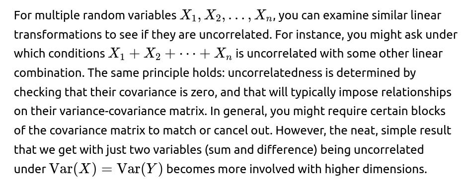
If X and Y are vector-valued random variables, how does the condition for uncorrelatedness of X+Y and X−Y extend to multiple dimensions?
When X and Y are vectors, say X ∈ ℝ^n and Y ∈ ℝ^n, we must consider their covariance matrices rather than single scalar variances. For two n-dimensional random vectors U and V, uncorrelatedness means their cross-covariance matrix is the zero matrix. Concretely, U = X + Y and V = X - Y are also n-dimensional random vectors, and they are uncorrelated if

In matrix form, their covariance is:
Cov(X+Y, X+Y) is the sum of Cov(X, X), Cov(X, Y), Cov(Y, X), Cov(Y, Y), etc.
Cov(X+Y, X-Y) expands to Cov(X, X) - Cov(X, Y) + Cov(Y, X) - Cov(Y, Y).
In the scalar case, we discovered that Var(X) − Var(Y) must be zero. For the vector case, that condition becomes:

where Σ_{XX} = Cov(X, X) is the covariance matrix of X, and Σ_{YY} = Cov(Y, Y) is the covariance matrix of Y. Therefore, for X+Y and X−Y to be uncorrelated component-wise, we need Σ_{XX} = Σ_{YY}.
A common pitfall arises when we assume the result “Var(X)=Var(Y)” in the scalar sense and blindly apply it to a vector scenario. Now we must match full covariance matrices: if the diagonal elements (variances of each coordinate) and off-diagonal elements (cross-covariances within each vector) all match, then X+Y and X−Y will be uncorrelated dimension by dimension. If only the diagonal entries match but the off-diagonals differ, the uncorrelatedness condition can fail because there may still be cross-component correlations that do not cancel out.
In real-world applications—e.g., in image processing or multivariate financial data—ensuring two vectors have identical covariance matrices can be nontrivial. The slightest mismatch in how each component correlates with others can break the uncorrelatedness. Therefore, to apply this condition in multidimensional settings, the entire covariance structure of X and Y must be identical, not just their overall “spread” in a single scalar sense.
Does the discrete or continuous nature of X and Y affect the condition for uncorrelatedness between X+Y and X−Y?
Uncorrelatedness in probability theory is defined through the covariance, which involves expectations (i.e., integrals or sums over the distribution). Whether X and Y follow discrete or continuous distributions, the derivation of Cov(X+Y, X−Y) = Var(X) − Var(Y) holds exactly the same. The key steps in the proof revolve around linearity of expectation and expanding expressions like (X+Y)(X−Y). None of these operations require X or Y to be continuous specifically; they merely require well-defined second moments (i.e., finite variances).
A practical pitfall is that in discrete distributions with heavy tails, the variance may be infinite or extremely large. In such cases, the notion of covariance might be undefined or highly unstable. If Var(X) or Var(Y) is infinite, we cannot even state the condition Var(X)=Var(Y). Hence, a crucial real-world edge case is verifying that both random variables have well-defined, finite variances. If they do, and those variances match, the result remains valid whether the distributions are discrete or continuous.
How do outliers or heavy-tailed distributions impact the ability to verify that Var(X)=Var(Y)?
Heavy-tailed or highly skewed distributions can make sample variance estimates very sensitive to outliers. When you try to estimate Var(X) and Var(Y) from finite data, a few extreme points can drastically shift the empirical variance. Consequently, in practice, you might incorrectly conclude that Var(X) ≠ Var(Y) if your sample is not large enough or if you have a few anomalous data points. Alternatively, you might overfit to a small dataset and find spurious equality of variances.
A subtlety here is that uncorrelatedness is about the true underlying distributions, not just estimates. With heavy-tailed data, you need robust statistical techniques—such as trimming or Winsorizing outliers, or using robust variance estimators—to get more reliable estimates of Var(X) and Var(Y). If those are close enough to be within some margin of estimation error, you might still conclude in practice that X+Y and X−Y are uncorrelated. However, you must remain cautious: a real possibility exists that additional data could reveal significant differences in variance. In financial data, for instance, rare but huge market moves can heavily influence variance and thus break the equality.
Does the condition Var(X)=Var(Y) impose any specific constraints on higher moments like skewness or kurtosis?
No, uncorrelatedness of X+Y and X−Y is determined solely by second-order statistics. Specifically, it depends only on Var(X) and Var(Y). Higher moments, such as skewness (third moment about the mean) or kurtosis (fourth moment about the mean), do not directly affect the covariance. Therefore, you can have distributions with wildly different skewness or kurtosis but the same variance, and still satisfy the condition that X+Y and X−Y have zero covariance.
However, just because these higher moments do not appear in the condition does not mean they cannot influence the broader relationship between X and Y. They could influence independence, tail dependencies, or other forms of non-linear correlation. But as far as the linear measure of uncorrelatedness is concerned, only the second moments come into play. This can be a pitfall if someone mistakenly interprets uncorrelatedness as an indication that the distributions are “similar” or that there are no other differences. Indeed, they may still differ significantly in shape and tail behavior.
If we scale X by a positive constant, how does that affect the uncorrelatedness of X+Y and X−Y?
Suppose we replace X with a scaled version aX, where a is a positive real constant. Then the sum and difference become (aX+Y) and (aX−Y). To check their covariance:
Var(aX) = a^2 Var(X).
Var(Y) remains the same if we do not scale Y.
Then Cov(aX+Y, aX−Y) = a^2 Var(X) − Var(Y). For these two new variables to be uncorrelated, we need a^2 Var(X) = Var(Y). If originally Var(X)=Var(Y), but then we apply a ≠ 1, that equality no longer holds unless we also change Y in a complementary manner.
Hence, scaling X alone changes the variance in a quadratic fashion. In practice, if you want to preserve the uncorrelatedness of the sum and difference after scaling, you would need to adjust both X and Y (or adjust your scale factors) to keep their variances identical. A common pitfall is applying some normalization (say, dividing X by its own standard deviation but not Y) and then expecting X+Y and X−Y to remain uncorrelated. That will break the condition unless Y undergoes a matching transformation.
How does this condition extend to time series data where X and Y are indexed over time?
When X and Y are time series (Xₜ, Yₜ), we can define the sum and difference at each time t as Uₜ = Xₜ + Yₜ and Vₜ = Xₜ − Yₜ. To analyze uncorrelatedness in a time series context, we must check

over time. The same algebra shows the instantaneous covariance for each t is Var(Xₜ) − Var(Yₜ). However, in time series analysis, we also look at autocovariance across different time lags. If we are only requiring pointwise uncorrelatedness (at the same time t), the condition remains Var(Xₜ)=Var(Yₜ) for each t. But if we consider cross-covariances at different lags—e.g., Cov(Uₜ, Vₜ₋ₗ) for some lag ℓ—the condition for uncorrelatedness might be more complicated.
Another subtlety is whether X and Y are stationary or nonstationary. In a stationary time series, Var(Xₜ) and Var(Yₜ) are the same for all t and might be estimated from a single sample path. If X and Y are nonstationary, their variances can change over time, so you could have Var(Xₜ)=Var(Yₜ) at one point in time but not at another. This can lead to partial or conditional uncorrelatedness at specific intervals. From a practical point of view, you would typically check the stationarity assumption first, then verify if the stationary distributions of X and Y share the same variance.
If X and Y are complex random variables, does the condition Var(X)=Var(Y) ensure uncorrelatedness of X+Y and X−Y?
Complex-valued random variables often handle covariance through Hermitian forms and consider quantities like E[(X+Y)(X−Y)*], where the * denotes complex conjugation. For real-valued variables, that conjugation does not change anything, but for complex variables, the notion of covariance typically generalizes to something akin to:

So you must ensure that the second moments line up appropriately in the complex plane. In many complex-valued random vector treatments (e.g., in signal processing for complex signals), we define separate covariance and pseudo-covariance terms to address real-imaginary correlations.
In simpler cases, if X and Y are zero-mean circularly symmetric complex Gaussians with identical variances, then X+Y and X−Y can indeed be uncorrelated in the sense of having zero cross-covariance. However, one subtlety arises if the imaginary parts have different variances or if there is a cross-term correlation between real and imaginary parts. Ensuring complete uncorrelatedness for complex variables might require matching not just the overall magnitude of variance but also the real-real, imag-imag, and real-imag covariance blocks. Hence, if X and Y are purely real or purely imaginary parts, the condition Var(X)=Var(Y) remains sufficient. But in the general complex case, one must be more diligent about how those second moments are structured.
What if the data for X and Y is partially missing or corrupted by measurement noise? How do we handle that in practice?
Real-world datasets often have missing entries or measurement noise superimposed on the true values of X and Y. If you try to estimate Var(X), Var(Y), and Cov(X+Y, X−Y) from such data, you face several complications:
Missing Data: You might have to discard rows where either X or Y is missing, or use an imputation technique. Discarding data can reduce sample size, harming statistical power. Imputing values can bias variance estimates unless done carefully (e.g., multiple imputation methods that preserve second moments).
Measurement Noise: If the observed X_obs = X + noiseₓ and Y_obs = Y + noiseᵧ, then Var(X_obs) = Var(X) + Var(noiseₓ) (assuming independence of X and the noise). Similarly for Y_obs. Even if X and Y had the same true variance, the presence of different noise variances can break that equality in the observed domain. That can cause an erroneous conclusion that X+Y and X−Y are correlated.
A robust approach might be to model noise explicitly, attempt to estimate or calibrate the noise variance, and then correct the observed sample variance accordingly (e.g., subtract out the known or estimated noise variance). Alternatively, use a maximum likelihood estimation for a parametric model that accounts for missingness and noise. A subtlety is ensuring that noise, X, and Y are independent or that we know how they correlate. If measurement noise correlates with X or Y in any way, that further complicates the analysis.
In practical scenarios, could boundary or domain constraints on X and Y invalidate the derivation?
Yes. If X and Y are defined over restricted domains (e.g., only nonnegative values, bounded intervals, or discrete sets where variance is impacted by a boundary effect), the standard approach to computing Var(X) and Var(Y) might still apply, but the distributions might exhibit strongly non-linear relationships. For example, if both X and Y are nonnegative random variables clipped at zero, there can be a mass at zero that skews the estimation of variance.
It is still true that the algebraic relationship

holds if the second moments exist. But domain constraints can lead to distortions in how one might interpret that covariance in real-world terms. If the domain restrictions lead to degenerate cases (e.g., X is bounded so that Var(X) → 0 under certain conditions), then the question of uncorrelatedness might reduce to trivial or degenerate outcomes. Always check that the domain constraints do not cause any violation of the assumptions behind computing second moments (finite, well-defined integrals or sums). If everything remains valid, the main formula still holds, but interpreting it requires caution.