ML Interview Q Series: Understanding R²: What Does 0.38 Mean for Your Regression Model's Performance?
📚 Browse the full ML Interview series here.
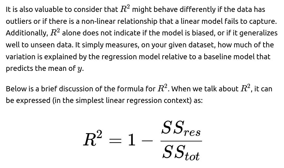
20. Regression problem R² = 0.38. What does this mean? How can you interpret it?
Check other error metrics such as RMSE (Root Mean Squared Error) or MAE (Mean Absolute Error). These metrics can reveal how large the typical error magnitude is in the same units as the target variable.
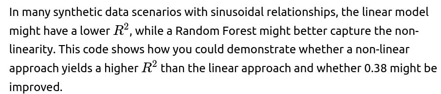
Investigate the possibility of non-linear transformations or more expressive models. If you suspect that the data has strong non-linear relationships, consider exploring more complex algorithms (like tree-based methods or neural networks).
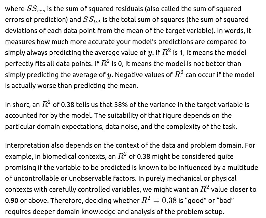
Evaluate domain trade-offs. In some scenarios, capturing 38% of the variance is sufficient to make meaningful decisions. In other scenarios, you may need to push for a higher level of explanation.

Practical example in Python
from sklearn.linear_model import LinearRegression
from sklearn.metrics import r2_score
import numpy as np

# Suppose we have some small synthetic dataset
X = np.array([[1], [2], [3], [4], [5]]).astype(float)
y = np.array([2.1, 2.9, 3.0, 4.1, 5.0]).astype(float)

model = LinearRegression()
model.fit(X, y)
predictions = model.predict(X)

r2 = r2_score(y, predictions)
print("R-squared:", r2)
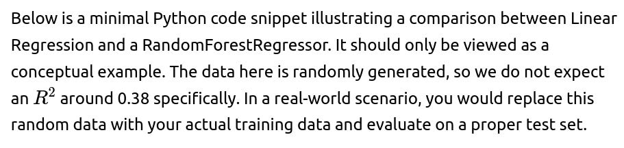
If this snippet outputs something around 0.38 (in practice, it will likely be higher for this trivial dataset), that means about 38% of the variance is explained by the model in that toy example context.

In a real-world scenario, you might suspect that your linear model fails to capture a more complex relationship among the features and the target. An interviewer could probe how you would respond to that. A strong response includes mentioning:
Exploring polynomial regression. For example, you might include polynomial terms of your predictors if domain knowledge or data exploration suggests a non-linear pattern.
Using more expressive models. Tree-based models (Random Forests, Gradient Boosted Trees) or neural networks can capture complex functions of the input features.
Performing feature engineering. If your features are not well-crafted or do not reflect the important transformations needed to capture relevant relationships, you might need domain-specific transformations or additional data sources.
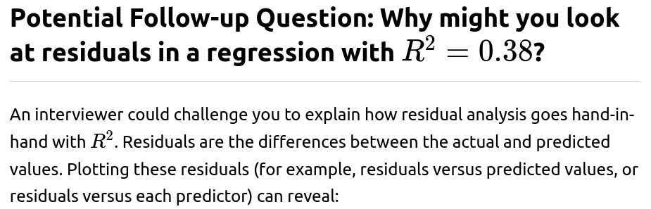
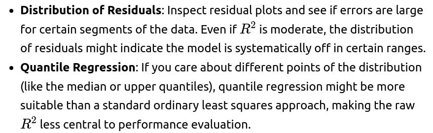
Checking residual plots. Plotting residuals against predicted values or against each feature can reveal systematic patterns that indicate non-linearity. If you see a strong curved shape in the residuals, that is a hint that a simple linear model may not be adequate.

One approach is to perform a thorough error analysis to see if the model is systematically missing certain patterns. Another approach is to collaborate with domain experts to find out if there are relevant features that are not currently part of your data. You might also:
Check for data quality issues or outliers that unduly influence model fits.
Explore more flexible model families. If you have only tried a simple linear model, you might try random forest regressors, gradient boosting regressors, or neural networks (depending on the size and complexity of data).
If domain experts indicate that your model underperforms known approaches, you can compare data sources, transformations, or modeling techniques they employed. You may also consider ensemble methods to combine several approaches to get higher performance.
Investigate new features. Collect additional data or transform existing features to capture subtle relationships.
Explore model complexity. Move beyond basic linear regression to polynomial regression, tree-based models, or neural networks if non-linear relationships are suspected.
Perform rigorous feature selection or regularization. Using L1 (Lasso) or L2 (Ridge) regularization can help manage overfitting while letting you systematically test expansions of feature sets.
Conduct error analysis to see if the model is missing certain clusters or subgroups of the data. For example, maybe your predictions are systematically poor for a specific sub-population in your dataset.
Experiment with ensemble methods such as Random Forest, XGBoost, or LightGBM, which can handle complex interactions effectively.
Using cross-validation. Splitting your data into multiple folds and computing an average performance metric across folds helps you see whether the model performance is consistent.
Avoiding “peeking” at the test set. Keeping a strict distinction between training/validation and test sets is critical to avoid inadvertently tuning the model based on test outcomes.

An interviewer might want to see if you can translate your technical understanding into simple language. One way is:
“Out of all the variability in our target outcome, our model can currently explain about 38% of it. That means we still have a significant portion—about 62% of it—unexplained. In more practical terms, if we use this model to predict the outcome, about 38% of the differences we see in real data can be predicted from the factors we include in the model, and the rest is still due to other unknown or unmodeled factors. Depending on our problem, this may or may not be sufficient. Let’s decide if that 38% helps us make better decisions than we would with no model at all, or if we need more features or a better approach.”
Such an explanation reflects an ability to communicate effectively with non-technical stakeholders.

import numpy as np
from sklearn.linear_model import LinearRegression
from sklearn.ensemble import RandomForestRegressor
from sklearn.metrics import r2_score
from sklearn.model_selection import train_test_split

# Generate synthetic data with some non-linearity
np.random.seed(42)
X = np.random.rand(100, 1) * 10
y = 3 * np.sin(X).ravel() + np.random.randn(100) * 0.5  # non-linear relationship

X_train, X_test, y_train, y_test = train_test_split(X, y, test_size=0.2, random_state=42)

lin_model = LinearRegression()
lin_model.fit(X_train, y_train)
lin_preds = lin_model.predict(X_test)

rf_model = RandomForestRegressor(n_estimators=100, random_state=42)
rf_model.fit(X_train, y_train)
rf_preds = rf_model.predict(X_test)

lin_r2 = r2_score(y_test, lin_preds)
rf_r2 = r2_score(y_test, rf_preds)

print("Linear Regression R^2:", lin_r2)
print("Random Forest R^2:", rf_r2)
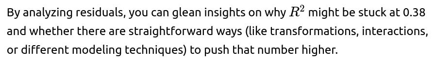
Patterns of non-linearity. If you see a curved trend, the relationship might not be linear.
Heteroscedasticity (unequal variance). If the spread of residuals grows for larger predicted values, that might violate assumptions of ordinary least squares.
Clustering or patterns by subgroups. You might discover that your model works very well for part of the dataset but systematically fails for another subset. This can drive you to engineer new features or build different models for different segments.
Sometimes domain-specific metrics can give deeper insight. For example, if you are predicting prices, you might consider percentage errors (like MAPE). If you are predicting time to an event in survival analysis, you might consider a measure like the concordance index. If you are predicting counts (like the number of events in a Poisson setting), you might look at deviance or mean deviance. If you are working on an energy demand forecasting problem, you might consider metrics that incorporate the cost or penalty of overestimation versus underestimation.
Below are additional follow-up questions
What is the difference between training set R² and test set R², and how should you handle it if there is a big gap?
Why might overfitting occur?
The model might be overly flexible (e.g., high-degree polynomial, large random forest, or deeply layered neural network).
The training set might not be diverse enough or representative.
Hyperparameters might be tuned specifically to the training set, neglecting generalization.
To handle this:
Does the scale of features or the target influence the R² value, and how might standardization affect its interpretation?
How can R² be misleading if the data is heavily skewed or unbalanced, and what are better approaches?
Better approaches or checks:
Look at multiple metrics: For skewed data, consider metrics like Median Absolute Error (MdAE) or Mean Absolute Percentage Error (MAPE), which can be more robust in reflecting typical errors.
Transformations: Log-transforming the target can mitigate skew. Then you can interpret how much variance in log(y) is explained. Always confirm that this is valid in your domain.
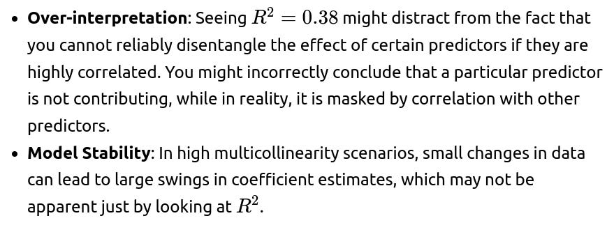
How might the presence of correlated features or multicollinearity affect the interpretation of R²?
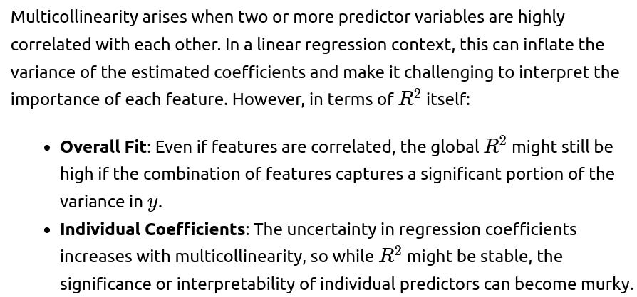
VIF (Variance Inflation Factor): In practice, you might measure VIF to detect multicollinearity. A high VIF indicates that the corresponding feature is strongly correlated with some combination of other features.
Pitfalls:
To mitigate:
Use regularization techniques (Ridge regression is often recommended if you have collinearity issues) because it penalizes large coefficients and helps maintain better numerical stability.
Consider dimensionality reduction (e.g., PCA) to remove redundancy among correlated features.
Could you explain how confidence intervals or hypothesis testing might be performed for R², and how that informs interpretation of R² = 0.38?
Why this helps:
A significant F-test can show that 0.38 is better than predicting the mean, but it doesn’t necessarily mean you have an excellent predictive model. It only shows there is some non-random explanatory power in your regression.
Pitfalls:
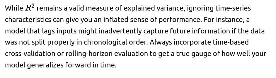
Does the notion of R² still hold in a time-series context, or would you do something else to measure performance?
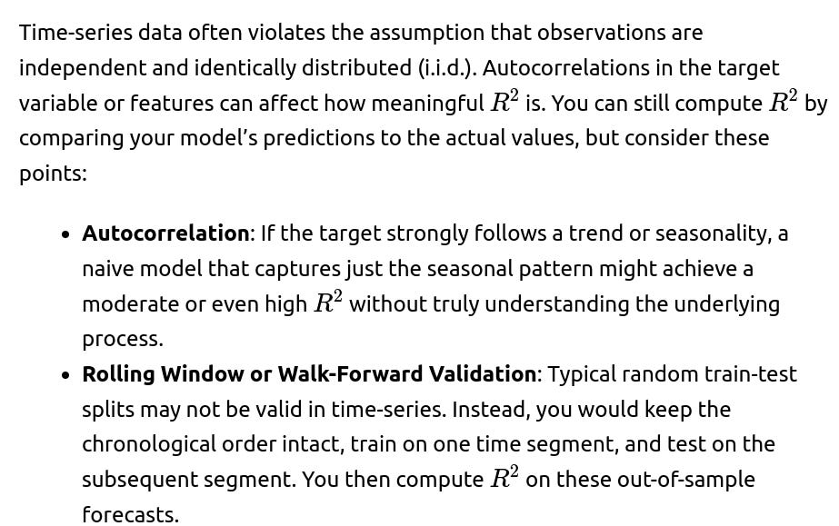
Alternative Metrics: Especially in time-series, metrics like the Mean Absolute Scaled Error (MASE) or the symmetric Mean Absolute Percentage Error (sMAPE) can sometimes be more revealing. They account for the scale and nature of time-series data.
If the data is extremely high-dimensional (p >> n), does R² still matter, or how do you adjust your perspective?
In a high-dimensional regime, you have many more features (p) than observations (n). This scenario can lead to:
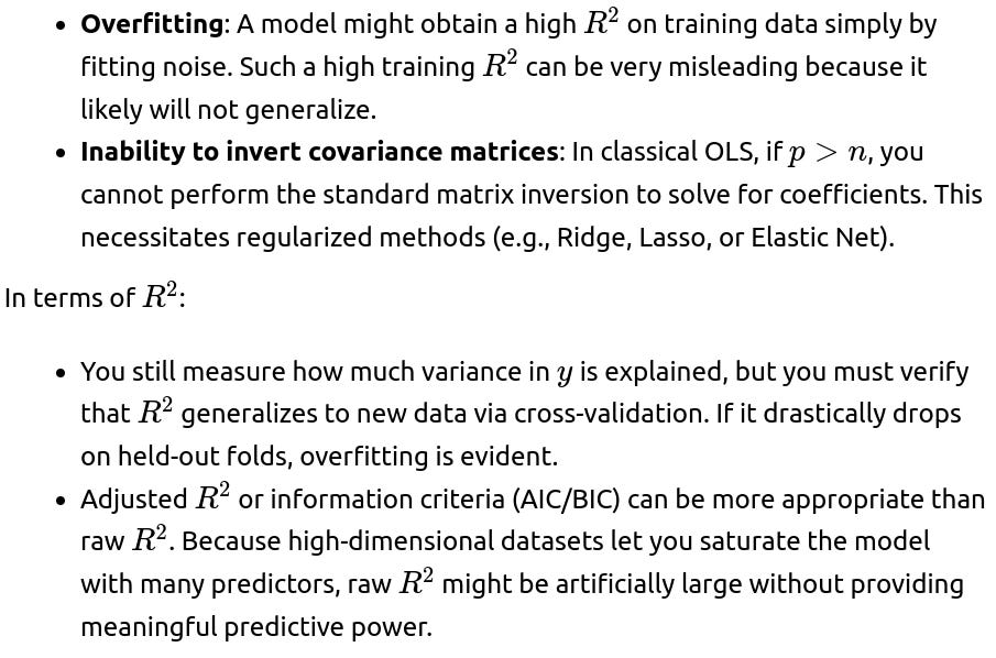
Practical adjustments:
Regularization is crucial. A simple linear regression with p>>n is usually not feasible without some penalty on coefficients.
Dimensionality Reduction (e.g., PCA or autoencoders) can reduce p before fitting a model, thereby avoiding the direct hazard of extremely high dimensional feature spaces.

In a real business scenario, how might partial R² for each feature be more informative than a single global R², and how is partial R² computed?

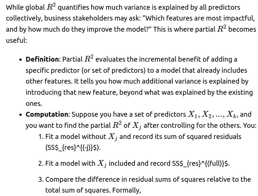
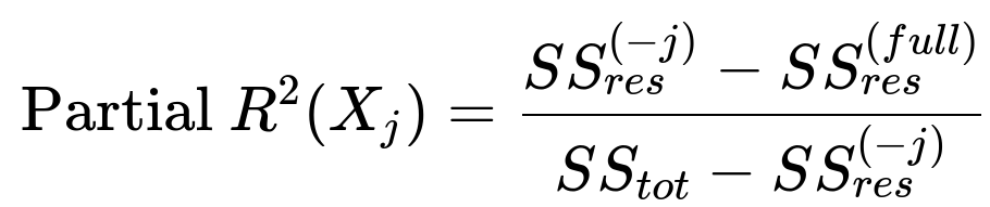
This formula can vary slightly based on the definition, but the main idea is to isolate the effect of adding that one feature.
In a business setting:
How might missing data or imputation methods affect R², and what special considerations should be taken?
Imputation: Common methods include mean imputation, median imputation, or model-based imputation (like KNN imputer or advanced methods such as MICE). While these approaches can preserve data size, they introduce potential biases:
If you impute in a simplistic way (e.g., constant value for all missing entries), you might artificially reduce variance in the dataset, affecting how you measure explained variance.
How do you weigh interpretability against achieving a certain R², and what strategies might you use?
Glass-Box Models: Sometimes, tree-based methods like gradient-boosted trees can offer feature importance scores. Although not as transparent as a small linear model, they can give partial dependence plots that illustrate how specific features influence predictions.
If an R² of 0.38 persists across multiple modeling attempts, how do you decide whether to continue improving the model or to move on?
Domain Requirements: If the application can meaningfully benefit from explaining at least 38% of the variability (for instance, if this is enough to reduce costs or make useful decisions), then the model may be acceptable. On the other hand, if the business or domain context demands explaining a higher fraction of variability or achieving a certain precision, you may need to do more.
Marginal Gains: If each new feature or modeling approach yields only tiny improvements, it might be time to consider that the phenomenon has a large unexplained component. Perhaps you lack crucial features that truly drive the outcome, or there is random noise inherent in the process that cannot be captured.
Exploratory Analysis of Residuals: Checking the patterns in the residuals can help you see if there is an entire sub-population or certain time period that is particularly poorly predicted. If so, a specialized model or additional domain-specific data might help.