
ML Interview Q Series: Uniform Conditional Distribution of an Exponential Variable Given a Fixed Sum

Browse all the Probability Interview Questions here.
Let X_1 and X_2 be independent random variables each having an exponential distribution with parameter μ. What is the conditional probability density function of X_1 given that X_1 + X_2 = s?
Short Compact solution
The conditional probability density function of X_1 given X_1 + X_2 = s is the uniform distribution on the interval (0, s). Concretely, for 0 < v < s,
f_{X_1 | X_1+X_2}(v | s) = 1/s,
and it is 0 otherwise.
Comprehensive Explanation
Setting up the problem
We have two independent random variables X_1 and X_2, each following an exponential distribution with the same rate parameter μ. This means that for i = 1 or 2, the probability density function (pdf) of X_i is:
f_{X_i}(x) = μ exp(-μ x) for x > 0, and 0 otherwise.
We are interested in the conditional pdf of X_1 given the event X_1 + X_2 = s (where s > 0 is a constant).
Defining V and W
A common strategy to tackle such problems is to define new random variables:
V = X_1
W = X_1 + X_2
We will use the joint distribution of (V, W) and then find the conditional density of V given W = s.
Joint pdf of (V, W)
Because V = X_1 and W = X_1 + X_2, we can write the inverse transformations:
v = V w = W x_1 = v x_2 = w - v
The Jacobian of this transformation is 1. We now compute the joint pdf f_{V,W}(v, w). For 0 < v < w,
f_{V,W}(v, w) = f_{X_1}(v) * f_{X_2}(w - v) = [μ exp(-μ v)] * [μ exp(-μ (w - v))] = μ² exp(-μ w).
Outside 0 < v < w (and w > 0), the joint pdf is 0.
Marginal pdf of W
To find f_W(w), we integrate out v from the joint pdf:
f_W(w) = ∫ f_{V,W}(v, w) dv, where the integral is from v = 0 to v = w.
Hence,
f_W(w) = ∫[0 to w] μ² exp(-μ w) dv = μ² exp(-μ w) * ∫[0 to w] dv = μ² exp(-μ w) * (w) = μ² w exp(-μ w), for w > 0.
This is recognized as the Erlang/Gamma distribution with shape parameter 2 and rate μ.
Conditional pdf of V given W = s
We use the general definition of conditional pdf:
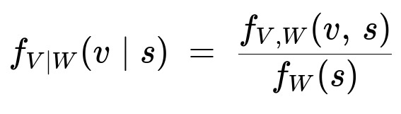
Substituting f_{V,W}(v, s) = μ² exp(-μ s) (for 0 < v < s) and f_W(s) = μ² s exp(-μ s) (for s > 0), we get
f_{V|W}(v | s) = [μ² exp(-μ s)] / [μ² s exp(-μ s)], for 0 < v < s.
Simplifying,
f_{V|W}(v | s) = 1 / s, for 0 < v < s.
And it is 0 otherwise. This shows that V = X_1, conditioned on the sum X_1 + X_2 = s, is uniformly distributed over (0, s).
Intuitive interpretation
The result can be understood from the fact that when you condition on X_1 + X_2 = s, there is no further “preference” for X_1 to take any specific value in (0, s). The uniform distribution naturally emerges due to the memoryless and exponential properties of X_1 and X_2.
Potential Follow-Up Questions
1) Why does conditioning on X_1 + X_2 = s yield a uniform distribution?
Because the exponential distribution is memoryless, when you specify the total sum s of two independent exponential random variables, each possible (X_1, X_2) pair that adds up to s is equally likely. This intuition can be confirmed by the formal derivation of the joint pdf and subsequent marginalization.
2) Does this result hold if X_1 and X_2 have different rate parameters?
No. The uniform result is specific to the case where X_1 and X_2 are i.i.d. exponentials with the same rate parameter. If they had different rate parameters, the conditional distribution would follow a different form (in fact, it would be a Beta-type distribution if one thinks of X_1 / (X_1 + X_2) rather than a strict uniform).
3) How can we simulate this scenario in Python?
Below is a simple code snippet to illustrate a simulation approach:
import numpy as np
import matplotlib.pyplot as plt

mu = 1.0
n_samples = 10_000_00

# Generate independent exponentials
X1 = np.random.exponential(scale=1/mu, size=n_samples)
X2 = np.random.exponential(scale=1/mu, size=n_samples)

# Compute sum
S = X1 + X2

# Condition on X1 + X2 = s (simulated by selecting samples close to some s)
s_target = 2.0
tolerance = 0.01
indices = np.where((S > s_target - tolerance) & (S < s_target + tolerance))[0]
X1_conditioned = X1[indices]

# Plot the histogram
plt.hist(X1_conditioned, bins=50, density=True, alpha=0.7, color='blue')
plt.title("Empirical Distribution of X1 | X1+X2 ≈ s")
plt.xlabel("X1")
plt.ylabel("Density")
plt.show()
By narrowing down S to be close to s_target, one can visualize how X1 is approximately uniform on (0, s_target) in the limit of large samples.
4) How do we interpret the memoryless property in this context?
The memoryless property states that for an exponential random variable X, P(X > a + b | X > a) = P(X > b). When we sum two exponential random variables with the same parameter, the ratio X_1 / (X_1 + X_2) turns out to be independent of the sum X_1 + X_2 and is uniformly distributed on (0, 1). This property is deeply tied to the uniform conditional distribution on (0, s) that we derived.
5) Could this concept extend to sums of more than two exponential variables?
Yes, if X_1, X_2, ..., X_n are i.i.d. exponentials with rate μ, then their sum follows a Gamma distribution with shape parameter n and rate μ. Conditioning on the sum, the joint distribution of (X_1, X_2, ..., X_n) given X_1 + ... + X_n = s follows a Dirichlet distribution (specifically the Dirichlet(1,1,...,1)). For n=2, the Dirichlet(1,1) is simply a uniform distribution on (0, s).
Below are additional follow-up questions
What if s is very close to zero or extremely large?
When s is extremely small (approaching 0), in principle, both X_1 and X_2 must be near 0 as well. However, the distribution of X_1 | (X_1 + X_2 = s) remains uniform on (0, s). For s very close to zero, the interval (0, s) is also very small, so X_1 will take values close to 0 almost surely. In practice, if we attempt to sample from this conditional distribution computationally, numerical precision can become a challenge because standard floating-point operations may struggle with extremely small intervals. Additionally, when s is extremely large, the uniform distribution (0, s) means that X_1 has a wide possible range of values, which might lead to numerical overflow when dealing with exponentials exp(-μ s) in certain computations. One must handle these edge cases (e.g., s = 0 is actually impossible since each exponential random variable is positive with probability 1, but numerically s can be very close to 0) carefully, possibly by using higher-precision arithmetic or robust sampling schemes.
How does the conditioning change if there is a small probability that X_1 or X_2 can be zero?
Strictly speaking, for continuous exponential random variables, the probability of exactly 0 is zero. Still, in real-world data collection, you could have truncated or discretized exponential measurements where an observation might occasionally be recorded as 0 if it falls below some sensor threshold. If either X_1 or X_2 can be exactly 0 with some probability (perhaps due to rounding or censoring in practice), the uniform distribution on (0, s) might no longer strictly hold. In that scenario, you would have additional probability mass concentrated at X_1 = 0 or X_2 = 0. If you detect any such zeros, you would need to alter the conditional density to reflect that some portion of the probability is allocated to the boundary. This could transform the problem into a mixture where part of the distribution remains uniform over (0, s), and part assigns probability to the boundary points.
Does the uniform conditional distribution hold if X_1 and X_2 have a correlation or dependence structure?
No. The derivation relies fundamentally on the independence of X_1 and X_2. If X_1 and X_2 share some positive or negative correlation (e.g., through a bivariate exponential distribution with a nontrivial dependence), then the conditional distribution f_{X_1 | X_1 + X_2 = s} will not remain uniform. For instance, if we impose a dependence structure such that when X_1 is large, X_2 tends to be smaller (or vice versa), then the uniform result is broken. The mathematics in that case would require integrating out the joint pdf that encodes the correlation term. Hence, a pitfall in applying the uniform conclusion in a real-world scenario is failing to check or test whether X_1 and X_2 are truly independent exponentials.
How do we handle truncated data in practice?
In many real-world scenarios, data might be truncated at some upper or lower threshold. For example, if measurements below a certain value are not recorded (left truncation) or beyond a certain value are censored (right truncation), the distribution of (X_1, X_2) is restricted. Then, even after conditioning on X_1 + X_2 = s, the resulting conditional distribution could differ from pure uniform. One typical approach is to re-normalize the density over the feasible truncated region and then derive a conditional pdf accordingly. The uniform property over (0, s) no longer holds once you have introduced constraints like “X_1 must exceed some minimum m > 0” or “X_2 cannot exceed some maximum M.” Proper likelihood-based treatments or specialized truncated/censored distribution formulas become necessary in these scenarios.
What if we look at functions of X_1 given X_1 + X_2 = s, such as X_1^k?
Sometimes we are not just interested in the distribution of X_1 itself but in transformations like X_1^k for some exponent k > 0. If X_1 is uniformly distributed on (0, s), then X_1^k will have its own distribution which can be determined by the usual change of variable approach for a uniform random variable. Specifically, for V = X_1^k with X_1 ~ Uniform(0, s), you can derive:
P(V <= v) = P(X_1^k <= v) = P(X_1 <= v^{1/k}),
and you must be sure that 0 < v^{1/k} < s. This helps in computing expectations of powers of X_1. For instance, E(X_1^k | X_1 + X_2 = s) becomes ∫ (from 0 to s) x^k (1/s) dx. These transformations are straightforward due to the simplicity of the uniform distribution, but if the underlying distribution were not uniform, the computation would be more involved.
What does the conditional result imply about the fraction X_1 / (X_1 + X_2)?
Because X_1 | (X_1 + X_2 = s) is uniform on (0, s), then X_1 / s is uniform on (0, 1). If you consider the ratio U = X_1 / (X_1 + X_2), that ratio is uniform on (0, 1) as well. A subtle point is that this uniform ratio phenomenon depends on X_1 and X_2 being i.i.d. exponentials. A pitfall might arise if one tries to apply the same ratio argument to different or correlated distributions. In that case, one might incorrectly assume U is uniform on (0, 1), which would be false if X_1, X_2 are not identically distributed exponentials with the same parameter.
How would one verify this uniform property empirically in a large-scale real-world dataset?
Empirical verification typically involves:
Collecting data points (X_1, X_2) that are known or assumed to be independent exponentials.
Grouping those points according to values of X_1 + X_2 within narrow bands around some s (e.g., pick a small interval [s - δ, s + δ]).
Examining the distribution of X_1 among all points for which X_1 + X_2 is in that interval. One might plot a histogram or run a goodness-of-fit test against the uniform distribution. A pitfall here is that if the sample size is not large enough or if the underlying assumptions (independence, identical rate parameters, truly exponential) fail, the histogram might deviate significantly from uniform. Moreover, real data could have outliers or be subject to sensor saturation (leading to floor/ceiling effects) that must be accounted for during this validation step.
Is there any geometric interpretation of the result?
Geometrically, if you plot the positive quadrant in the (x_1, x_2) plane, the condition X_1 + X_2 = s corresponds to a line segment that stretches from (0, s) to (s, 0). For independent exponentials with the same rate, the probability density is proportional to exp(-μ (x_1 + x_2)). Conditioning on being exactly on that line (i.e., x_1 + x_2 = s) causes all points on the line between (0, s) and (s, 0) to be “equally likely” in the limit. One subtlety is that a small part of the plane near x_1 + x_2 = s could have slightly different densities if we don’t condition exactly; in practice, though, the uniform distribution is exact only for the strict condition. A pitfall in any geometric or intuitive argument is forgetting that we need to integrate over the entire support to confirm uniformity, not just rely on a purely geometric measure of distance or length.