
ML Interview Q Series: Uniform Point Sampling in a Circle Using Inverse Transform Sampling

Browse all the Probability Interview Questions here.
How can you sample points uniformly at random inside a circle of radius R?
Short Compact solution
A direct way is to use an inverse-transform approach on the radius and independently sample a uniform angle. If you denote the radius by r, its probability density function is
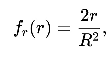
valid over the interval from 0 to R. The cumulative distribution function is
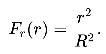
If you draw a random variable y from a Uniform(0,1) distribution, set
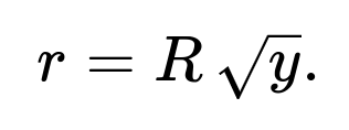
Then choose an angle θ uniformly on [0, 2π). Convert these polar coordinates to Cartesian coordinates as
x = r cos(θ)
y = r sin(θ)
to obtain uniformly distributed points in the circle of radius R.
Comprehensive Explanation
Why the radius must be sampled via the square root of a uniform variable
When picking a point uniformly inside a circle, we want each infinitesimal area element to have the same probability of being chosen. The area of a thin annulus at distance r from the origin is proportional to r (since the circumference of a circle of radius r is proportional to r, and the annulus thickness is a small increment in radius). Hence, the chance of landing in that annulus increases with r. Mathematically, the fraction of the total area corresponding to all points with radius less than or equal to r is
Area of a circle of radius r: πr²
Area of the full circle of radius R: πR²
So the cumulative probability to be within radius r is (r²)/(R²). That leads to a distribution for r of (r²)/(R²). If y ~ Uniform(0,1), equating y = (r²)/(R²) gives r = R√y. This accounts for the fact that points further out in the circle occupy more area and thus must be sampled more frequently than points near the center.
Why we choose the angle uniformly
The uniformity requirement applies to all orientations around the center. In polar coordinates, the angle θ ranges from 0 to 2π. To ensure points are evenly distributed in all directions, choose θ ~ Uniform(0, 2π). This approach guarantees rotational symmetry.
Pitfalls if you try something else
If you naively choose r ~ Uniform(0, R) and θ ~ Uniform(0, 2π), you get more points clustered near the origin because the area coverage at smaller radii is smaller. That would not be uniform in terms of area. The correct method requires sampling r with the distribution proportional to r, which is effectively r = R√y, as described.
Example Implementation in Python
import numpy as np

def sample_points_in_circle(num_points, R=1.0):
    # Sample uniform(0,1) for radial component
    u = np.random.rand(num_points)
    # Sample uniform angle in [0, 2*pi)
    theta = 2 * np.pi * np.random.rand(num_points)

    # Convert to correct radius distribution
    r = R * np.sqrt(u)

    # Convert to Cartesian
    x = r * np.cos(theta)
    y = r * np.sin(theta)

    return x, y

# Example usage:
x_coords, y_coords = sample_points_in_circle(num_points=10000, R=2.0)
This code generates 10,000 points uniformly distributed within a circle of radius 2. The logic corresponds exactly to the formula described above.
Potential Follow-up Question 1
Why do we use the relationship r = R√y instead of picking r from Uniform(0, R)?
A uniform draw of r between 0 and R would lead to more samples in the center, since each concentric ring from r to r+dr must contain roughly 2πr × dr area. A uniform selection of r means you are ignoring the fact that outer rings have larger circumference and hence more area. Using the square root ensures every area segment has equal sampling probability.
Potential Follow-up Question 2
What if we just sample points in the square [−R,R] × [−R,R] and discard points that are outside the circle?
This rejection method is also valid for uniform sampling in a circle, but it might be less efficient because many draws in the outer corners of the square are discarded. The ratio of accepted points to total points generated in this method is πR² / (2R)² = π/4 ≈ 0.785, so about 21.5% of samples in the square end up discarded. For larger dimensions (e.g., hyperspheres), rejection sampling becomes even more wasteful.
Potential Follow-up Question 3
How do you generalize this procedure to higher dimensions?
In higher dimensions (e.g., sampling uniformly in an n-dimensional ball), you can:
Generate n independent standard normal random variables (to get a random direction) and normalize that vector.
Generate a radius with the appropriate distribution for the n-dimensional volume element. In n dimensions, the radius r has a distribution such that the volume scales with r^(n−1). The function for the radius in n dimensions involves the inverse of the integrated volume fraction.
This ensures that every n-dimensional “shell” is sampled in proportion to its hyper-volume.
Potential Follow-up Question 4
Can we directly choose random polar coordinates in 2D with a simpler approach?
One might consider polar coordinates with r chosen from uniform(0,R). That is not correct for uniform sampling in terms of area, for reasons mentioned above. The correct approach always accounts for how the area grows with r, giving the required pdf for r proportional to r in 2D.
Potential Follow-up Question 5
What numerical stability concerns might arise in practice?
If R is very large or you are performing calculations on a GPU or specialized hardware, floating-point precision might come into play when squaring or taking square roots.
In typical double-precision floating-point, this rarely causes major issues for standard ranges of R. However, in extremely large or small scales, rounding errors could accumulate and you may need higher-precision libraries or scaling transformations.
These potential numerical issues are usually minor for most practical circles.
Below are additional follow-up questions
How does the method change if the circle is not centered at the origin?
The sampling method remains fundamentally the same, but after generating the point’s polar coordinates (r, θ) and converting them to Cartesian coordinates, you must shift the resulting (x, y) by the circle’s center location. If the circle is centered at (x₀, y₀) rather than (0, 0), you would produce:
x' = x₀ + r cos(θ) y' = y₀ + r sin(θ).
The main pitfall arises if you forget to translate the points or if you incorrectly transform the radius distribution based on some offset. The uniform distribution logic does not change; only the final coordinates need the shift. In large-scale simulations, it is common to center many circles differently, and mixing up coordinate frames can cause subtle bugs if translations are applied incorrectly.
How can we check if our sampling is truly uniform in practice?
An effective approach is to perform statistical goodness-of-fit tests or visual diagnostics. One method is to generate a large number of sampled points and then:
Partition the circle into a grid of sub-regions (like concentric rings, or small wedges) and count how many points fall into each region.
Compare the empirical counts against what a uniform distribution would predict for those regions.
You can also compute the distances of your sampled points from the center. The distribution of those radii should match the theoretical distribution r = R√y, or equivalently, the radii-squared should be uniformly distributed in [0, R²]. Potential pitfalls include small sample sizes (which can obscure the uniformity) and random number generator deficiencies that can create clumps or patterns. Ensuring a well-tested pseudorandom generator and a sufficiently large number of points helps confirm uniformity.
If we transform or scale coordinates after sampling, does the distribution remain uniform?
Uniformity in the original circle remains valid as long as transformations do not alter the relative areas of regions in a way that distorts the distribution. For example, if you merely shift all sampled points by a constant vector, the distribution is still uniform but centered at the new location. If you apply a uniform scaling factor to both axes (turning a circle of radius R into a circle of radius kR), that retains uniformity within the new circle.
However, a non-uniform scaling (e.g., scaling x- and y-axes differently) transforms the circle into an ellipse, and the sampling is no longer uniform with respect to the ellipse’s area. In that scenario, you need a different approach to preserve uniformity in the ellipse domain. A subtle pitfall arises if you accidentally treat expansions differently on the x and y axes, assuming uniformity still holds when it does not.
In parallel computing environments, how do we maintain independence across multiple threads or workers?
Each thread or worker must have its own independent source of randomness, usually by initializing distinct random number generator states. Care must be taken that two different workers do not accidentally share seeds. A common pitfall is forgetting to seed separate generators properly, causing identical streams of random numbers in each thread and producing repeated samples.
Another subtle issue is ensuring the random draws remain uncorrelated when combined. If the same seed is used across workers, the entire point set may follow a repetitive pattern, undermining uniformity. The standard remedy is to use either a high-quality parallel random number library or generate a master random seed for each thread in a reproducible but disjoint way.
How do we handle sampling in an annulus, where we only want points between an inner radius r₁ and an outer radius r₂?
One way is to sample the radius from a distribution that spans r₁ to r₂ but still accounts for the area difference. The probability of landing in the annulus up to some radius r (where r₁ ≤ r ≤ r₂) is proportional to the area difference:
Area fraction = (πr² − πr₁²) / (πr₂² − πr₁²).
When you set a uniform variable y in [0, 1], you solve for r in
r² = r₁² + y(r₂² − r₁²).
Hence:
r = √[r₁² + y(r₂² − r₁²)].
The angle θ is still drawn from 0 to 2π uniformly. Pitfalls include forgetting that you must exclude the area inside the inner radius or inadvertently using the formula for a full circle from 0 to R. Implementation errors often arise if you do not carefully differentiate between total circle area and the annular area.
In real-world implementations, could the quality of the random number generator degrade the uniformity?
Yes. Certain pseudorandom number generators (PRNGs) have shorter periods or patterns that can cause non-uniform clustering over large sample sizes. If the PRNG is not well-suited for scientific simulations, correlations or repeated sequences can appear. To mitigate this, use trusted libraries and PRNGs with robust statistical properties (e.g., Mersenne Twister or hardware-based random number sources for critical applications). For extremely large simulations, seed cycling or suboptimal generator states can lead to subtle biases. Frequent validation checks and using proven libraries help minimize these risks.
Are there ways to sample within arbitrary shapes using bounding shapes or advanced algorithms?
Yes. One general approach for arbitrary shapes is rejection sampling with a bounding region. You sample uniformly in a simple shape (like a rectangle or circle) that encloses the target region and then keep only those points lying inside the shape of interest. However, if the shape is complicated or has a lot of empty space in the bounding region, this can be highly inefficient.
More sophisticated methods include adaptive subdivision of the region into smaller bounding shapes, Monte Carlo methods with partial knowledge of shape boundaries, or specialized algorithms like the “hit-and-run” approach for high-dimensional convex bodies. The key pitfall is balancing simplicity of implementation versus computational efficiency, especially in complex or high-dimensional domains where rejection sampling can become prohibitively expensive.