
ML Interview Q Series: Uniform Variables: PMF of First Exceedance Index via Conditional Probability

Browse all the Probability Interview Questions here.
Let X_1, X_2, … be independent random variables uniformly distributed on (0,1). The random variable N is defined as the smallest n ≥ 2 for which X_n > X_1. What is the probability mass function of N?
Short Compact solution
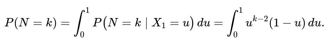
By conditioning on X_1 = u, the distribution of N given X_1 = u is a shifted geometric with success probability p = 1 - u. Hence:

which evaluates to

The expected value is infinite, i.e. E(N) = ∞.
Comprehensive Explanation
To find the probability mass function (pmf) of N, we start by observing that N is the first index n ≥ 2 for which X_n > X_1. Here, X_1, X_2, … are independent and uniformly distributed on (0,1).
Step-by-step reasoning
Distribution of X_1: Since X_1 is uniform on (0,1), it takes values in (0,1) with equal likelihood.
Condition on X_1 = u: After we see that X_1 = u, we look for the first n ≥ 2 such that X_n > u. Because each X_n is uniform on (0,1) and independent of X_1, the probability that a given X_n exceeds u is (1 - u). Consequently, the process of searching for the first X_n > u (for n ≥ 2) behaves like a geometric process, but it is “shifted” by the fact that we start counting from n=2 instead of n=1. Specifically, if N is the first index ≥ 2 for which X_n > u, then N - 1 is geometric with parameter (1 - u). So:
P(N = k | X_1 = u) = (u)^(k-2) (1 - u), for k = 2, 3, …
because we need X_2, …, X_{k-1} all to be ≤ u (probability u each), and X_k to be > u.
Integrate out X_1: To get the unconditional distribution, we integrate over all possible values of X_1:
Evaluate the integral: The integral ∫ from 0 to 1 of u^(k-2)(1 - u) du can be recognized as a Beta function integral. Alternatively, one can do direct integration. Either way, the result is:
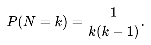
Support for k: This pmf holds for k = 2, 3, … since N is defined to be at least 2.
Infinite expected value: It turns out that N has no finite mean. By substituting P(N = k) = 1 / [ k (k-1 ) ] into the sum for the expectation, one sees that the sum ∑ from k=2 to ∞ of k · P(N = k) diverges. Hence E(N) = ∞.
In summary, the probability mass function is 1 / [ k(k-1 ) ] for k ≥ 2, and the expected value diverges.
What does it mean that P(N = k) = 1 / [ k(k-1 ) ]?
It means that for each integer k ≥ 2, the probability that the first index n ≥ 2 with X_n > X_1 is k decreases on the order of 1 / k^2. This is a heavy tail that sums to 1 but whose associated expectation diverges.
Potential Follow-up Questions
Why is E(N) infinite despite the pmf summing to 1?
When a distribution’s tail is heavy enough, its pmf can sum to 1 while the series for the mean diverges. Specifically, the pmf behaves like a constant times 1 / k^2 for large k, which is just borderline enough that its harmonic-like series for k * (1 / k^2) behaves like 1 / k and diverges in the infinite limit.
Could we have recognized the integral more quickly?
Yes. One might note that u^(k-2)(1-u) from u=0 to 1 is closely related to the Beta function B(a,b) = ∫ from 0 to 1 of t^(a-1)(1-t)^(b-1) dt. In this case, a = k - 1 and b = 2. The Beta function B(k-1, 2) evaluates to Γ(k-1)Γ(2)/Γ(k+1). Using factorial expressions for integer arguments yields 1 / [ k(k-1 ) ].
Are there alternative derivations of P(N = k)?
Yes. A quick argument without direct integration is to notice:
X_1 takes some value u in (0,1).
N = k if X_2, …, X_{k-1} ≤ u and X_k > u.
By symmetry and independence, the probability that the rank of X_1 among (X_1, …, X_k) is exactly r is 1 / k for any r = 1, 2, …, k. For N = k, X_1 must be the largest among X_1, …, X_{k-1} but smaller than X_k. Carefully accounting for that ordering yields the same pmf 1 / [ k(k-1 ) ].
How might you quickly verify these probabilities in practice?
You can run a Monte Carlo simulation:
import numpy as np

def simulate_probability(num_samples=10_000_000):
    counts = {}
    for _ in range(num_samples):
        x1 = np.random.rand()
        n = 2
        while True:
            x = np.random.rand()
            if x > x1:
                counts[n] = counts.get(n, 0) + 1
                break
            n += 1
    for k in sorted(counts.keys()):
        print(k, counts[k] / num_samples)

simulate_probability()
As num_samples grows, the empirical frequency of each N=k will approximate 1 / [ k (k-1 ) ].
Are there any practical implications of having an infinite expectation?
In certain practical scenarios, an infinite expectation implies that although the probability of very large values of N is small, it is not negligible enough to ensure a finite mean. This warns us that waiting times governed by such distributions can grow disproportionately large in rare events, which has implications for system design, load handling, and performance guarantees.
Below are additional follow-up questions
Could there be any real-world scenarios where you encounter infinite expected values, and how do you handle them?
An important real-world scenario involves waiting times in certain queueing systems or reaction times in random processes. If you see that the distribution of the waiting time has a “heavy” or “fat” tail, the mean might diverge. Handling such a scenario typically requires:
Robust system design: Because rare events can happen that result in extremely large values, systems must be over-provisioned or built with fallback mechanisms (e.g., timeouts, parallelization) to mitigate the impact of huge waiting times.
Alternative performance metrics: Rather than relying on the mean (which is infinite), one might look at quantiles (like the median) or tail bounds (like Value at Risk or Conditional Value at Risk in finance) that give a better representation of typical or “worst-case” scenarios in day-to-day operations.
A potential pitfall is to assume that everything with a finite probability distribution has a finite mean and then design a system that relies on average-case analysis. This can be disastrous if the true mean is infinite, leading to drastically underestimated resource requirements.
How does the Law of Large Numbers behave if you sample N repeatedly?
If you treat N as a random variable itself and take many independent draws from its distribution, you might expect that the sample average approaches the theoretical mean. However, in this case, E(N) is infinite. The Strong Law of Large Numbers only guarantees convergence to the mean if the mean is finite. With an infinite mean, the sample average of repeated measurements of N does not converge to a finite number; in fact, it tends to grow unbounded. A subtlety here is that in finite samples, you will sometimes see moderate sample averages, but occasionally an extremely large N will appear and significantly shift the average.
Pitfall: Believing one can gather enough samples to “estimate the mean” precisely can be misleading if the mean is infinite. Empirical estimates will fluctuate wildly due to extremely large outlier observations.
How would you check if the pmf is valid and indeed sums to 1?
You can verify that the sum of 1 / [k(k-1)] from k=2 to infinity converges to 1 as follows. Notice that:
1 / [k(k-1)] = 1 / (k-1) - 1 / k
This is a telescoping series. Written out explicitly from k=2 up to some large K,
(1/1 - 1/2) + (1/2 - 1/3) + (1/3 - 1/4) + … + (1/(K-1) - 1/K) = 1 - 1/K
As K → ∞, this sum tends to 1. So the pmf is valid. A common mistake is to see the 1 / k^2 behavior and jump to the wrong conclusion that it might not sum to 1 or might sum to something less or more. Recognizing the telescoping nature resolves this quickly.
Why is it essential that the random variables X_1, X_2, … are i.i.d. Uniform(0,1)?
The definition of N relies on comparing X_n with X_1 and requiring the first X_n to exceed X_1. If the distribution were not independent, the event X_n > X_1 might be correlated across n. If the distribution were not uniform, the probability that X_n > X_1 would not simply be (1 - X_1). For instance, if the X_n had some non-uniform distribution, the conditional distribution could be very different or more involved to compute. In short, i.i.d. Uniform(0,1) gives a direct handle on the probability that one sample is bigger than another sample (just the difference 1 - u).
A common pitfall is to assume that the result 1 / [k(k-1)] generalizes to other distributions or to dependent samples without carefully checking those assumptions. That assumption breakdown can lead to incorrect pmfs.
What if we consider the variance of N?
Since E(N) is infinite, higher moments such as the variance and even second moments become ill-defined in the usual sense (they would also be infinite). Sometimes you can still examine the tail distribution to infer certain properties, but for typical notions of variance, it does not exist (it is also infinite). A misconception would be to claim that if the pmf sums to 1, the variance must be finite. This is not true; summing to 1 is only a requirement for a pmf to be valid, not for its moments to be finite.
What happens if we define a truncated version of N?
A truncated version might be something like min(N, T) for some fixed cutoff T. This ensures we never measure N beyond T and might be used in practical simulations to avoid unbounded runs. If we do that, the expected value of min(N, T) is finite because it cannot exceed T, but it departs from the original distribution for large values. In some algorithmic contexts, you might put a cap on how long you wait before timing out.
The subtlety is that truncation changes the distribution’s tail and eliminates that infinite-mean characteristic. So you no longer have the same random variable, but for practical engineering scenarios, it can be necessary to keep computations stable and bounded.
How does one interpret the meaning of "the smallest n ≥ 2 for which X_n > X_1" in practical modeling?
In real-world settings, it can be seen as a problem of “rank detection.” Suppose you have an initial sample X_1 (like a reference measurement) and you keep drawing new samples X_2, X_3, …, looking for the first time you exceed the baseline X_1. The index N captures how many tries you need before you see a value larger than the original. In some contexts, this can represent:
The first day’s price is a reference, and N is the first day with a higher price.
The first test outcome is a baseline, and N is the first test that improves upon this outcome.
A misunderstanding might be assuming that exceeding X_1 is highly likely to happen quickly. In many runs, it does happen early, but there remains a significant probability that it takes a very large number of tries, making the average unbounded.
What if we wanted to modify the definition of N to "N is the smallest n ≥ 2 for which X_n < X_1"? Would the distribution change?
Yes. If N is defined as the first index n ≥ 2 for which X_n < X_1, the reasoning changes symmetrically. We would then have the success probability p = u when conditioning on X_1 = u, because we want X_n to be less than u. That would lead to:
P(N = k | X_1 = u) = (1-u)^(k-2) * u
and the pmf upon integrating out X_1 = u would likely have a similar form but reflect that p = u. One might do the integral:
∫ from 0 to 1 (1-u)^(k-2) * u du
and discover the same telescoping style that results in 1 / [k(k-1)]. So the distribution is effectively the same, just a mirror interpretation. The pitfall here is to assume that reversing the condition “> X_1” to “< X_1” drastically changes the distribution. Because of symmetry in the uniform (0,1) distribution, it does not.
How might the result differ if N was defined as "the smallest n ≥ 2 for which X_n = X_1"?
Since X_1 and X_n are continuous Uniform(0,1), the probability that X_n equals X_1 exactly is 0 for any n. Thus, the event “X_n = X_1” has probability 0 for each n, and with countably infinite draws, the probability remains 0 in an i.i.d. continuous setting. This implies N would be almost surely infinite. In practice, we say that the probability that all X_n differ from X_1 is 1, meaning that you will never find an n ≥ 2 with X_n exactly equal to X_1 in an ideal continuous model. A real-world subtlety is floating-point representation or measurement precision. If you measure to finite precision, collisions can occur with some positive probability. This is a classic example of how theoretical continuous assumptions might differ from computational realities.
Can we view this problem from an order-statistics perspective and how does that help?
Yes. By considering the order statistics of the first k samples (X_1, X_2, …, X_k), you can see that X_1 has an equal probability of being the smallest, second smallest, …, largest among these k samples. In general, the probability that X_1 is the r-th order statistic among X_1, X_2, …, X_k is 1 / k for each r = 1, …, k. For the event N = k to happen, X_1 must be at least as large as all of X_2, …, X_{k-1}, but smaller than X_k. Carefully tracking these ordering events leads to the same 1 / [k(k-1)]. This perspective can simplify the algebra by leveraging known facts about the distribution of order statistics for i.i.d. uniform variables. A typical pitfall is to rely on more complex conditioning arguments, while a simple symmetry or rank argument might be faster and less error-prone.