ML Interview Q Series: Using Custom Error Metrics for Imbalanced Data with Asymmetric Misclassification Costs.

Jun 08, 2025

📚 Browse the full ML Interview series here.

42. Consider a dataset with 90% negative points and 10% positive points, where misclassifying a positive point as negative is very costly compared to misclassifying a negative as positive. Which error metric is more appropriate?

a) Balance the data and then use Accuracy b) F1 Score c) A custom error metric like a × |type1 errors| + b × |type2 errors|, with a >> b d) AUC

A custom error metric (option c) is more appropriate. This is because misclassifying a positive point (often referred to as a Type II error or false negative) is far more costly in this scenario, and a custom error metric with a much larger penalty for false negatives can directly reflect this real-world cost in your model evaluation and optimization process.

Below is a detailed explanation of why this is the correct choice, along with a deeper discussion of the other metrics and the reasons they may be less appropriate under these specific circumstances. After that, several follow-up questions are presented (in H2 format), each followed by thorough answers and additional insights.

Why a Custom Error Metric Best Suits This Scenario

A custom error metric like

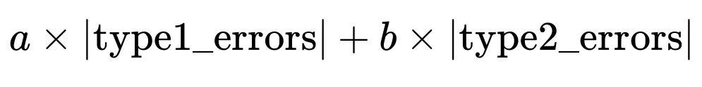
where you set a much larger weight for false negatives (type2 errors) than false positives (type1 errors), directly encodes the high cost of missing a positive. In many real-world settings, such as detecting fraudulent transactions or critical medical diagnoses, missing a single positive instance (a real fraud, or a real illness) can be far more detrimental than flagging a negative instance incorrectly.

Type I error = false positive = misclassifying a negative as a positive Type II error = false negative = misclassifying a positive as a negative

If a >> b, the cost function penalizes false negatives much more aggressively. For example, if a model incorrectly classifies a positive example as negative, the term a × |type2_errors| will add a large cost, forcing the optimization process to shift its decision boundary to reduce false negatives.

Detailed Reasoning About Other Options

Balancing the data and using Accuracy

Balancing the data artificially (by undersampling or oversampling) and then using accuracy alone can still obscure the difference between the two types of mistakes. Even if the classes are balanced during training, the accuracy metric does not inherently weight false negatives differently from false positives. If misclassifying a positive is much worse than misclassifying a negative, accuracy alone will not focus on punishing those costly errors sufficiently.

F1 Score

F1 Score is the harmonic mean of precision and recall. It partially addresses class imbalance by focusing on the performance for the positive class (precision and recall both revolve around the positive class). But F1 Score still treats false positives and false negatives with a certain symmetry: maximizing F1 tries to balance precision and recall, rather than explicitly giving extra emphasis to one type of error if that error is far more costly in the real world. While F1 is more appropriate than accuracy for imbalanced classification, it does not offer the precise control that a custom loss function or custom error metric provides for punishing false negatives more severely.

AUC (Area Under the ROC Curve)

AUC measures how well a model can separate positives from negatives across various thresholds. It is useful for comparing general separation capability, but it does not directly reflect a real cost structure where false negatives might be far more critical than false positives. A model could have a reasonably high AUC yet still produce an unacceptably high number of false negatives if it sets a particular threshold. In practice, you might use the ROC curve or the Precision-Recall curve to find a good threshold, but if you already know that false negatives are disproportionately costly, you can make that cost structure explicit in a custom metric or in the training objective.

Key Insights

A custom error metric is a very direct way to embody domain-specific costs. While F1 Score, Accuracy, and AUC can provide important insights, none of them inherently let you specify "a >> b" to heavily penalize false negatives. By incorporating the higher cost of misclassifying positives directly into the model selection or model training process (for instance, weighting the loss function accordingly or using a custom decision threshold derived from that cost), you ensure that the model’s performance is aligned with the real-world impacts of its mistakes.

Follow-up Question: Why Not Simply Use F1 Score to Handle the Imbalance?

F1 Score is certainly more robust than accuracy on imbalanced datasets, because it accounts for both precision and recall. However, it does not explicitly differentiate the relative cost of false negatives versus false positives. If you know that missing a positive (false negative) is much more serious, you want to explicitly push your model to reduce those false negatives, potentially at the expense of tolerating more false positives.

F1 Score aims to find a balance between precision and recall. It treats them with equal importance. If you need to place greater emphasis on recall (to reduce false negatives), you could consider a metric like the F2 score, which weighs recall more heavily:

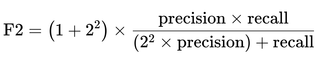
But even that might not fully reflect your specific real-world cost ratio unless it precisely matches the relative costs you face. A custom error metric is often the most transparent and flexible solution because it can be tailored to the exact ratio of cost.

Follow-up Question: How Do We Implement This Custom Error Metric in Practice?

One common practical approach is to incorporate class weights or a cost matrix directly in the loss function during training, if your framework supports it. For instance, in a classification context:

If you are using a cross-entropy loss in PyTorch, you can assign a higher weight to the positive class. For example:

import torch
import torch.nn as nn

# Suppose we have 2 classes, 0 (negative) and 1 (positive)
# We want to assign a large weight to the positive class
weights = torch.tensor([1.0, 5.0])  # example: weigh class 1 five times more
criterion = nn.CrossEntropyLoss(weight=weights)

Another approach is to compute a cost-based metric after predictions are made. For instance:

def custom_cost(preds, targets, a, b):
    # preds: predicted labels (0 or 1)
    # targets: true labels (0 or 1)
    # a: cost of false negative
    # b: cost of false positive
    type1_errors = 0  # false positives
    type2_errors = 0  # false negatives

    for p, t in zip(preds, targets):
        if p == 1 and t == 0:
            type1_errors += 1
        elif p == 0 and t == 1:
            type2_errors += 1

    return a * type2_errors + b * type1_errors

In this way, you can experiment with different values of a and b and choose the ratio that best represents your real-world cost scenario. During training, you might also use a validation set to track this cost metric and pick the model (or threshold) that yields the minimal custom cost.

Follow-up Question: Could We Just Modify the Decision Threshold Instead of a Custom Metric?

Adjusting the decision threshold is a simpler approach to achieve higher recall (thus fewer false negatives). For instance, if your model outputs probabilities for the positive class, you can set a threshold lower than the default 0.5 to label an instance as positive. This typically increases the detection rate of positives (reducing false negatives) but also increases false positives.

However, adjusting the threshold alone still does not directly encode the true costs unless you systematically evaluate different thresholds using a cost-based metric. You might sweep the threshold from 0 to 1, calculate the false positive rate and false negative rate at each step, and then compute the custom cost. Whichever threshold yields the lowest overall cost is your operational threshold. So while threshold tuning can help, you still need a cost function (or something that captures the same idea) to quantify what is “optimal” in your domain.

Follow-up Question: How Do We Choose Values for a and b?

Choosing a and b often comes from domain expertise. Some considerations include:

Financial impact. For example, if each missed positive might cost $10,000, while a false positive might cost $100, you might set a=100 and b=1.
Regulatory or safety reasons. If a false negative could lead to a severe safety issue or regulatory penalty, you might set a extremely large relative to b.
Empirical experimentation. You can try different ratios of a:b on a validation or test set and see which ratio best aligns with real-world outcomes (such as profit, safety margins, or user satisfaction).

In sum, the exact values usually come from the real-world environment, domain constraints, or a cost analysis. There is typically no single universal ratio, so it is important to work closely with domain stakeholders (e.g., finance experts, doctors, product teams) to set these penalty parameters appropriately.

Follow-up Question: Why Is Accuracy Particularly Misleading in Imbalanced Settings?

When the data is heavily skewed (like 90% negative and 10% positive), a trivial model that always predicts “negative” will achieve 90% accuracy. Clearly, that does not solve the underlying problem of identifying positive instances, which are the minority but costlier to miss. Accuracy does not tell you how well your model handles the minority class, especially when misclassifications of that class have a high cost.

In real-world scenarios where positives are rare, but extremely important to detect, accuracy can be dangerously deceptive. It masks the failure to detect positives behind the large proportion of correctly identified negatives. This is why we often look at metrics like Precision, Recall, F1, or custom cost-based metrics in addition to (or instead of) raw accuracy.

Follow-up Question: What About AUC? Isn’t It Good for Imbalanced Datasets?

AUC (Area Under the ROC Curve) does measure how well your model ranks positive and negative samples overall, and can be helpful when datasets are imbalanced. But it still does not differentiate between the costs of false positives and false negatives. A model could have a good AUC if it generally separates the classes well but might still produce too many false negatives if the chosen threshold is not well aligned with your cost preferences.

In some applications, the Precision-Recall (PR) curve and the area under that curve (Average Precision) can be more insightful for heavily imbalanced problems, especially when the focus is on correctly identifying the rare class. However, even Precision-Recall curves do not inherently incorporate the domain-specific cost structure. They simply provide an aggregate view of precision and recall across thresholds. To truly capture the idea of “missing a positive is super costly,” you still need a direct cost-based approach or at least an approach that is strictly recall-focused if that’s the crucial element of your problem.

Follow-up Question: Are There Pitfalls with Using a Custom Error Metric?

One pitfall is that if you heavily penalize false negatives, your model might become extremely conservative, flagging many negatives as positives just to avoid missing any true positives. This can lead to a large number of false positives, which might overwhelm downstream systems or lead to user frustration (for example, too many fraudulent alerts that are not actually fraud). Another subtlety is how to correctly choose or calibrate a and b so they reflect true real-world costs.

If the chosen penalty values are not realistic, you might push your model in a direction that does not match the real environment. Therefore, it is often best to consult domain experts, use real cost estimates, or at least carefully tune and experiment with different penalty weights on validation sets.

Follow-up Question: How Could We Explain This Choice to Non-Technical Stakeholders?

It can be helpful to frame the discussion in terms of real cost or real impact, which resonates more with non-technical audiences:

Emphasize that your model has two types of mistakes: failing to detect a positive case (false negative) or incorrectly marking a negative as positive (false positive).
Explain that missing a positive is much worse for the business or for safety reasons, so you penalize that error more in your evaluation.
Show them a chart of how many positives you expect to miss and how many false alarms you generate at a given threshold, highlighting the trade-off.

By presenting your analysis of what each mistake costs the organization and how you reflect that cost in your model training or evaluation, non-technical stakeholders typically become more comfortable with the custom approach.

Follow-up Question: Does Weighting the Classes in a Loss Function Always Lead to the Same Results as a Custom Error Metric?

Weighting the classes in a standard loss function (such as weighted cross-entropy) is a common approximation of having a custom error metric. In many cases, it can yield similar outcomes, but it does not always match perfectly for several reasons:

Class weights in the loss function influence how the model’s parameters are updated at each training step. However, the ultimate decision threshold for classification might still need separate tuning.
A custom metric like a × |type1_errors| + b × |type2_errors| can be evaluated post hoc on any set of predictions. The internal training process might not fully optimize for that metric unless it is integrated directly into the training objective or used to select a threshold on the output probabilities.
Some loss functions can be more sensitive to weights than others, and there might be practical constraints (like exploding gradients if the weights are extremely high).

Hence, while weighting is a powerful tool, you typically still want to measure actual performance via your custom metric on a validation set to select an appropriate threshold or finalize your model choice.

Follow-up Question: Could AUC or F1 Still Be Used in Parallel?

Yes, you might track multiple metrics during development:

Monitor F1 or recall to ensure you are capturing a sufficient proportion of positives.
Monitor a custom cost metric to see if the model is hitting your cost-based objectives.
Monitor AUC or precision-recall curves if they help you quickly compare different model architectures.

Different metrics highlight different aspects of model performance. In many real settings, showing a variety of metrics helps reveal the strengths and weaknesses of each candidate model. But the final decision or the most critical guiding metric in your scenario is the custom cost-based metric that best captures the actual stakes of each type of error.

Follow-up Question: In Summary, How Should One Answer an Interview Question About a Metric for Costly False Negatives?

The best approach in an interview is to emphasize that when one type of error (false negative) is more expensive or risky, you want a metric that directly encodes that higher penalty. That is precisely what a custom error metric does. Mentioning that you can do this either:

By designing a custom loss function that incorporates those costs.
Or by setting a custom evaluation function and searching for a threshold that minimizes it.

And explain that metrics like Accuracy, F1, or AUC do not explicitly capture the cost difference between false positives and false negatives. They can be helpful as secondary metrics, but they are not as directly aligned with the real-world cost structure as a custom metric that has a >> b when false negatives are more critical.

This demonstrates to the interviewer that you not only understand the standard metrics but also how to adapt them (or create new ones) for real-world applications where different errors have different consequences.

Below are additional follow-up questions

How do we handle model validation and cross-validation when using a custom cost metric?

When using a custom cost metric, you should integrate it into every step of your model selection process, including cross-validation. Traditionally, cross-validation uses a standard metric like accuracy, precision, recall, or F1. If you care more about false negatives than false positives, none of these standard metrics fully captures that. So you can:

Replace or augment your default validation metric with your custom cost metric.
Perform k-fold cross-validation, compute the custom cost on each fold, and average the results. This helps ensure the custom metric is robust to variance across different subsets of data.
Still keep track of other metrics (e.g., recall, precision, or F1) if you want a more holistic view. But the driving metric for deciding which model or hyperparameters to choose should be the custom cost.

Pitfalls and subtle issues can arise, such as:

If the cost metric heavily penalizes false negatives, the model might learn to flag nearly everything as positive in some folds, leading to an inflated cost on the flipside for false positives. You may observe high variance in your cross-validation folds if the minority class is sparse.
You need to ensure that the folds maintain the same class distribution, especially if the data is highly imbalanced. Otherwise, your cost estimates per fold could be inconsistent.
The custom cost might be sensitive to your chosen decision threshold if your model produces probabilities. You might have to do threshold tuning for each fold to find the minimal cost. That can be computationally expensive but typically yields a more accurate measure of real-world performance.

Can the cost ratio a >> b shift over time, and how would you handle dynamic changes in real-world costs?

Real-world costs are often dynamic. For instance, in fraud detection, the cost of a missed fraudulent transaction might rise if fraudsters become more sophisticated, or the tolerance for false alarms might decline if users are complaining. When these ratios shift, you need to revisit your model’s threshold or retrain the model with updated class weights or cost parameters:

If you are tracking your cost ratio in a system that updates over time (e.g., monthly or quarterly cost reviews), you can re-run your training or threshold-tuning process with the revised ratio.
In an online learning or streaming environment, you might dynamically adjust the threshold based on the latest known cost ratio. If your model outputs probabilities, you can pick the threshold that optimizes the new cost function in near real-time.

Potential edge cases:

If the cost flips dramatically (e.g., from false negatives being extremely costly to false positives suddenly being more costly), your model might need a complete retraining strategy. A small threshold tweak might not suffice.
You must ensure that your pipeline for collecting cost or feedback data is reliable. Over- or underestimating cost can lead to suboptimal performance.
If the cost is highly volatile, you risk chasing short-term fluctuations. Sometimes it is beneficial to choose a stable cost ratio that approximates the average scenario, so you are not perpetually re-optimizing and confusing upstream or downstream processes.

How can we address multi-class classification scenarios where each class has different misclassification costs?

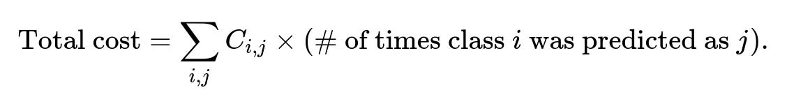
In multi-class classification, each class might have its own cost for being misclassified. For example, missing a certain disease could be extremely expensive, while mislabeling a benign condition as something serious might be less costly. You can extend the binary cost function to a matrix:

C = [ [0, C(1,2), ..., C(1,K)],
      [C(2,1), 0, ..., C(2,K)],
      ...,
      [C(K,1), C(K,2), ..., 0] ]

where (C_{i,j}) is the cost of misclassifying a true class i as class j. You can then compute a total cost:

To implement this:

During training, you can set class-specific weights if your framework supports it, or you can explicitly incorporate a custom loss function that references this cost matrix.
At inference time, for each sample, you can estimate the cost of assigning it to each class, then pick the class that yields the lowest expected cost.

Pitfalls include:

The cost matrix must be carefully determined. If the domain is complex (e.g., multiple medical conditions), obtaining accurate cost estimates for each pair of classes can be nontrivial.
The complexity of threshold tuning or cost-based decision rules can increase significantly as you move from binary classification to K-class classification.
Data imbalance across multiple classes can introduce additional challenges, requiring specialized sampling or weighting approaches.

Are there off-the-shelf algorithms that inherently handle cost-sensitive classification without explicitly defining a custom metric?

There are cost-sensitive learning algorithms that accept cost matrices or class weights directly. Some examples:

Certain decision tree implementations can use a cost matrix to adjust splitting criteria.
Gradient boosting frameworks (e.g., XGBoost, LightGBM) allow you to specify scale_pos_weight or more advanced approaches to incorporate cost.
Support Vector Machines can adjust cost parameters via class weights.

However, these built-in approaches are still essentially a simplified means of encoding a custom metric or objective. You often do not get as much flexibility compared to writing your own custom objective or performing post-hoc threshold optimization against your custom cost.

Edge cases:

Some frameworks only allow a single weight per class, not a full matrix for multi-class problems. This might not fully capture nuanced misclassification costs.
If you push the class weights to extreme values, the algorithm might become unstable or produce degenerate results, such as labeling almost everything as the high-cost class.

What strategies exist for extremely rare classes (e.g., 0.1% positives) when false negatives are extremely costly?

When the minority class is extremely rare yet critically important:

You can implement specialized sampling techniques, such as oversampling the minority class (e.g., SMOTE) or undersampling the majority class. Although you lose some data, it may help the model learn to identify positives more effectively.
You can use anomaly detection techniques if the positive events are extremely unusual. Models like isolation forests or one-class SVMs might do well, but typically you still want to embed the cost structure in your final evaluation and threshold decisions.
You can incorporate domain knowledge or rule-based pre-filtering so that the model only inspects a subset of data. For instance, if you know certain patterns are highly indicative of the rare event, focusing the model on that subset can improve detection.

Potential pitfalls:

SMOTE or other synthetic oversampling methods might produce unrealistic synthetic points that do not reflect real positives, especially if the positives are extremely rare and varied.
Very low prevalence can cause the model’s outputs to be poorly calibrated for higher thresholds. You might need more advanced calibration strategies to get probability estimates that are meaningful.
Even a small absolute number of missed positives could be disastrous. That means your cost ratio might be extremely high, risking a scenario where the model floods you with false positives.

What if the model outputs continuous scores rather than probabilistic estimates? How do we apply the custom cost?

Sometimes a model produces continuous decision values that are not naturally in the [0,1] range (e.g., margin outputs from SVM). You can still find a threshold or map these values to a probability-like scale via logistic calibration or Platt scaling. Then, once you have a “score” in [0,1], you can:

Sweep the threshold from 0 to 1 in small increments.
For each threshold, classify instances as positive or negative.
Compute your custom cost for that threshold.
Pick the threshold that yields the lowest cost.

Alternatively, if you want the model to directly optimize for cost, you can incorporate custom training procedures that handle the raw scores. However, the more common approach is to produce a probability-like output and apply cost-based threshold selection post hoc.

Edge cases:

If the model’s scores are poorly calibrated, picking a threshold based on cost can yield suboptimal results. Proper calibration methods (e.g., isotonic regression) might help.
In real-time systems with streaming data, sweeping thresholds might be too expensive. You can do a one-time or periodic threshold search on a recent batch of labeled data, then apply that threshold going forward.

How do we address interpretability when using a custom cost metric?

When you heavily penalize false negatives, your model might make decisions that differ significantly from traditional “balanced” models. Stakeholders might ask why so many predictions are flagged positive or why the cost-based strategy is favored over a simpler metric like F1. To enhance interpretability:

Provide confusion matrices under the chosen threshold and highlight the difference in total cost for that threshold vs. a baseline threshold (like 0.5).
Visualize cost curves. Plot your model’s custom cost vs. threshold. Show how the cost changes as you become more or less conservative with predictions.
If using a model with feature importance (e.g., random forests, gradient boosting), you can still measure which features drive the predictions that avoid false negatives. Clarify that the custom cost “pushes” the model to emphasize certain signals.

Potential pitfalls:

Interpretability can become more challenging if your approach is a black-box neural network or a complex ensemble. If the domain requires explainable AI (e.g., healthcare or finance), consider simpler models or incorporate explainability methods (SHAP, LIME).
Users might misunderstand the rationale for penalizing false negatives so heavily. Clear communication about real-world consequences is necessary.

What are potential data drift issues with a cost-sensitive approach?

Data drift is when the distribution of the incoming data changes over time. This can be particularly problematic in a cost-sensitive setup because:

Your custom cost or weighting scheme may have been tuned for historical data distribution. As the data changes, the ratio of positives to negatives or the features predictive of the positive class could shift.
A model that was carefully calibrated with a certain cost ratio might become suboptimal or misaligned as new patterns emerge in real-world data.

To mitigate this:

Continuously monitor performance metrics (including your custom cost) on fresh data.
Periodically retrain or fine-tune the model using the latest data. If the cost ratio is stable but the data distribution is changing, you may still need to adjust the decision threshold.
Consider an online or incremental learning algorithm that updates in real time.

Edge cases:

If you do not have timely labels for the positive class (e.g., in certain fraud scenarios, it might take a long time to confirm fraud), you could be slow to detect that the positive distribution has changed.
Rare but emerging patterns might go unnoticed, leading to a sudden spike in cost if the model misses a new variant of a positive case.

Could ensemble methods reduce the risk of over-penalizing one type of error?

Ensemble methods, like bagging or boosting, can help mitigate some of the extremes when you heavily penalize false negatives. By averaging or aggregating multiple models’ predictions, you might get more stable performance. For instance:

In boosting (e.g., XGBoost), you can incorporate a custom objective function or weighting scheme. Each weak learner focuses on mistakes made by the previous learners, so if false negatives are heavily penalized, the ensemble tries to reduce them cumulatively.
In bagging (e.g., random forests), each tree might handle the imbalance or cost weighting slightly differently, but the aggregate prediction can improve overall balance between false negatives and false positives.

Pitfalls:

If your weighting or cost ratio is extremely high, all ensemble components might converge to the same conservative strategy of labeling nearly everything as positive.
Overfitting can still occur if the ensemble is very large or if the minority class distribution is extremely small. Even an ensemble might not see enough positive examples to generalize well.
You still need to pick the final threshold that balances the cost. Ensembles do not inherently solve threshold selection.

How does one handle the scenario where misclassification costs are not strictly numerical, but more qualitative?

Sometimes the “cost” is not a precise dollar figure or a strict numeric penalty. For instance, reputational damage, legal risk, or emotional harm might be intangible. Even so, you can approximate these with a numeric scale to represent different severity levels. For example:

A “critical” misclassification might have a cost of 1000.
A “serious” one might have 100.
A “minor inconvenience” might have 1.

Then you can apply the same methodology: define a custom metric that sums up those costs across all misclassifications. Although it is approximate, it at least captures the idea that some mistakes are drastically worse than others.

Potential edge cases:

If stakeholders strongly disagree on how to quantify intangible costs, your model might face contradictory requests. Reaching consensus can be an organizational challenge rather than a purely technical one.
Overly simplistic numeric approximations might lead you to undervalue or overvalue certain mistakes. If possible, gather real user feedback or historical examples to anchor these costs more concretely.

How can we incorporate active learning or human-in-the-loop approaches in cost-sensitive environments?

In high-cost misclassification scenarios, it may help to have humans review certain borderline cases:

You can set a probability threshold range (e.g., predictions with probabilities between 0.4 and 0.6) as “uncertain,” and then route these to a human for review. This helps reduce severe false negatives or false positives when the model is unsure.
Over time, the labeled data from human reviews can be fed back into the model, improving it in future iterations.
You might define a cost not only for the misclassifications but also for the time or resources spent on human reviews. This leads to a more holistic cost metric that balances the expense of human oversight against the cost of errors.

Pitfalls and subtleties:

If your data volume is huge, you might not have enough human resources to review all uncertain cases. Deciding which cases are genuinely worth review is a design problem.
Humans can also make mistakes, especially if the domain is complex (like rare medical diagnoses). Incorporating the cost of human error is another layer of complexity.
Over-reliance on human-in-the-loop approaches might prevent the model from standing on its own if that is your end goal.

Rohan's Bytes

Discussion about this post