ML Interview Q Series: Using Linearity of Expectation & Combinatorics for Random Subset Overlap Analysis

Browse all the Probability Interview Questions here.

9. Alice and Bob are choosing their top 3 shows from a list of 50 shows. Assume they choose independently and randomly. What is the expected number of shows they have in common, and what is the probability that they do not have any shows in common?

This problem was asked by Disney.

To explore this question comprehensively, we will break down the key points, reasoning steps, and potential follow-up questions that might be asked in an in-depth machine learning or general quantitative interview setting. We will also provide relevant explanations of the combinatorial logic and probability concepts involved. Below, you'll find detailed answers that reflect the kind of depth FANG companies often expect during interviews.

Understanding the Scenario:

• Alice randomly chooses her top 3 shows from a list of 50.

• Bob also independently chooses his top 3 shows from the same list of 50.

• We are interested in:

  • The expected (average) number of shows they have in common.

  • The probability that they have zero shows in common.

Expected Number of Shows in Common

To find the expected number of common shows, we leverage the linearity of expectation. The key idea is that for each of the 50 shows, we consider the event "that show is chosen by both Alice and Bob."

Defining the event:

• For each show (say Show ( i )), define an indicator random variable ( X_i ) such that:

  • ( X_i = 1 ) if Show ( i ) is chosen by both Alice and Bob,

  • ( X_i = 0 ) otherwise.

Number of shows in common:

• Let ( X ) = total number of common shows = ( X_1 + X_2 + \dots + X_{50} ).

Expected value via linearity of expectation:

• ( E(X) = E(X_1 + X_2 + \dots + X_{50}) = E(X_1) + E(X_2) + \dots + E(X_{50}). )

Probability that a given show ( i ) is chosen by both:

• Alice chooses 3 out of 50 at random, so the probability that show ( i ) is in Alice’s selection is ( \frac{3}{50} ).

• Similarly, Bob chooses 3 out of 50 at random (independently), so the probability that show ( i ) is also in Bob’s selection is ( \frac{3}{50} ).

• By independence, ( P(\text{show i is chosen by both}) = \frac{3}{50} \times \frac{3}{50} = \frac{9}{2500}. )

Hence,

• ( E(X_i) = \frac{9}{2500}. )

Therefore,

• ( E(X) = \sum_{i=1}^{50} E(X_i) = 50 \times \frac{9}{2500} = \frac{450}{2500} = \frac{9}{50} = 0.18. )

So the expected number of shows in common is ( \frac{9}{50} ) (which is approximately 0.18).

Probability That They Have No Shows in Common

We now want the probability that all 3 shows Alice picks and all 3 shows Bob picks are disjoint sets, i.e., no overlap at all.

Using a combinatorial argument:

• The total number of ways Alice can pick 3 shows out of 50 is ( \binom{50}{3} ).

• Once Alice has chosen her 3 shows, Bob must choose his 3 shows from the remaining 47 shows to have zero overlap with Alice’s picks.

• The number of ways Bob can choose 3 out of the 47 that Alice didn’t pick is ( \binom{47}{3} ).

Hence, the probability of no overlap is:

We can write it explicitly as:

• Numerator: ( \binom{47}{3} = \frac{47 \times 46 \times 45}{3 \times 2 \times 1} = 16215. )

• Denominator: ( \binom{50}{3} = \frac{50 \times 49 \times 48}{3 \times 2 \times 1} = 19600. )

Thus, the probability of no shows in common is:

So they have about an 82.73% chance of picking completely disjoint sets of 3 shows.

Putting It All Together:

• Expected number of shows in common: ( 0.18 ) (or exactly ( \frac{9}{50} )).

• Probability that there are zero shows in common: ( \frac{\binom{47}{3}}{\binom{50}{3}} \approx 0.8273. )

Below, we address likely follow-up questions an interviewer might pose, along with detailed, in-depth answers to each.

Follow-up Question: How would these results change if each person chose shows with different probabilities (i.e., not uniformly at random)?

If Alice and Bob do not each choose their top 3 uniformly from 50, the logic changes in two core ways:

First, Expected Number of Common Shows:

• The simple factor ( \frac{3}{50} ) for each show no longer holds if some shows are more likely to be picked than others. Suppose each show ( i ) has a probability ( p_i ) that Alice picks it, and a probability ( q_i ) that Bob picks it, with the constraint that each must pick exactly 3. This can become more complex if the probability distribution is not uniform or if it enforces "exactly 3 shows" with varying probabilities.

• In that scenario, the probability that a given show ( i ) is chosen by both is ( p_i \times q_i ). Summing across all shows, the expected number of common shows is:

• However, if there's a constraint that exactly 3 are chosen by each person but with different preference weights, you would need to consider a more involved combinatorial or weighted approach. The uniform assumption simplifies the problem significantly.

Second, Probability of No Common Shows:

• The uniform assumption (i.e., all (\binom{50}{3}) subsets equally likely) breaks down if some shows are chosen with higher probability. Instead of a neat combinatorial ratio ( \frac{\binom{47}{3}}{\binom{50}{3}} ), you would compute:

• where ( S_A ) is the 3-show set Alice picks, and ( S_B ) is the 3-show set Bob picks, and ( P(S_A), P(S_B) ) reflect the new probability distributions. This is typically more cumbersome to compute exactly unless there's a known structure (e.g., a known preference weighting).

Follow-up Question: Can you show how to quickly verify these probabilities with a short Python simulation?

Yes. A quick Monte Carlo simulation can validate the analytical results. Although in an interview setting you might not always have time or permission to code, showing an example can emphasize your practical understanding. Below is a concise example in Python:

import random
import math
import numpy as np

def simulate(num_trials=10_000_00):
    no_overlap_count = 0
    common_counts = []

    for _ in range(num_trials):
        # Alice's picks
        alice_picks = set(random.sample(range(50), 3))
        # Bob's picks
        bob_picks = set(random.sample(range(50), 3))

        common = alice_picks.intersection(bob_picks)
        common_counts.append(len(common))

        if len(common) == 0:
            no_overlap_count += 1

    avg_common = np.mean(common_counts)
    prob_no_overlap = no_overlap_count / num_trials
    return avg_common, prob_no_overlap

if __name__ == "__main__":
    avg_common, prob_no_overlap = simulate()
    print(f"Estimated average #common: {avg_common}")
    print(f"Estimated prob of no overlap: {prob_no_overlap}")

Explanation:

• We repeat the random selection process many times (num_trials).

• Each trial, we pick 3 unique shows for Alice and Bob from the range 0 to 49.

• We count the intersection size (common chosen shows).

• After many trials, we compute the average intersection size (this should approach the theoretical value of 0.18).

• We also compute the fraction of trials that have zero overlap (this should approach about 0.8273).

Follow-up Question: Why does the linearity of expectation approach work so nicely for the expected number of common shows?

Linearity of expectation states that for random variables ( X ) and ( Y ),

regardless of any dependencies that might exist. In our case, even though the events "Show 1 is picked" and "Show 2 is picked" can be correlated (because each person can only pick 3), the expected value of the sum of indicators still decomposes as a simple sum of their individual expectations. This property dramatically simplifies many probability computations, including those involving overlaps or intersections of sets.

Follow-up Question: How would we adjust the probability of no overlap if Alice and Bob pick different numbers of shows (say Alice picks 3, Bob picks 5)?

In that scenario, the steps are conceptually similar but with different combinatorial factors:

1. Number of ways Alice picks 3 from 50: ( \binom{50}{3} ).

2. Number of ways Bob picks 5 from 50: ( \binom{50}{5} ) if Bob is also uniform random among all 5-sized subsets.

3. Probability that Bob has zero overlap with Alice’s 3 picks:

   • First, pick Alice’s 3 from 50, then Bob must pick 5 from the remaining 47. So the count of valid ways is ( \binom{47}{5} ).

   • The probability of no overlap is ( \frac{\binom{47}{5}}{\binom{50}{5}}. )

This straightforwardly generalizes the concept of “no overlap” to any chosen subset sizes.

Follow-up Question: What if we needed the probability that Alice and Bob share at least ( k ) shows? How would we compute that?

To compute "share at least ( k )" shows, you can sum over all the ways they can share exactly ( j ) shows for ( j = k, k+1, \dots, \min(3,3) ) in the case that each picks exactly 3. For each fixed ( j ):

1. Choose ( j ) common shows out of 50: ( \binom{50}{j} ).

2. Then Alice must choose ( 3-j ) distinct shows out of the remaining ( 50-j ). That can be done in ( \binom{50 - j}{3 - j} ) ways.

3. Bob must choose ( 3-j ) distinct shows out of the remaining ( 50 - j ). That can also be done in ( \binom{50 - j}{3 - j} ) ways, but note that we must be careful to avoid double-counting because once the j common shows are set aside, Alice picks from the remaining pool, Bob also picks from the same remaining pool.

4. The total number of ways to pick any 3 shows for Alice is ( \binom{50}{3} ), and the same for Bob is ( \binom{50}{3} ), but usually in such problems, we consider the total pairs of 3-element subsets of a 50-element set, which is ( \binom{50}{3} \times \binom{50}{3} ). Alternatively, if you approach it from the perspective “Alice picks 3, then Bob picks 3,” you’d keep the denominator as ( \binom{50}{3} ) for Bob’s sets given a fixed choice for Alice.

5. Sum from ( j = k ) to ( j = 3 ) (since the maximum overlap is 3).

This is a more involved combinatorial sum, but the principle remains: break it down into “how many ways to have exactly ( j ) in common” and then sum over all relevant ( j ).

Follow-up Question: What subtle mistakes might candidates make when doing these probability questions?

1. Mixing Up Permutations and Combinations

   • Sometimes, candidates will forget we are talking about subsets (combinations) rather than ordered selections (permutations). In these problems, the order in which Alice or Bob picks the shows does not matter.

2. Misapplying Independence

   • When computing the probability of “no overlap,” one must be careful about whether sets are chosen independently. Although Alice’s choice is independent of Bob’s, the events “Bob picks some specific subset of shows” might not be simply multiplied out if we were using the same sample space incorrectly. The combinatorial ratio handles this properly.

3. Failing to Simplify the Combinatorial Expressions

   • Interviewers often look for a neat ratio ( \frac{\binom{47}{3}}{\binom{50}{3}} ). Some might attempt more complicated expansions and confuse themselves by partial expansions.

4. Not Realizing How to Use Linearity of Expectation

   • A common pitfall is trying to count the overlap in complicated ways, missing that linearity of expectation trivially solves the “expected overlap” with minimal fuss.

5. Numerically Incorrect Computations

   • Small arithmetic mistakes (like incorrectly computing (\binom{47}{3})) can lead to incorrect final probabilities. Double-checking or simplifying carefully is crucial, especially under interview pressure.

Follow-up Question: How might the results be interpreted in a real-world scenario?

Imagine 50 possible popular TV shows. Two random viewers, Alice and Bob, each watch exactly 3 shows completely at random from the entire set:

• On average, they’ll share about 0.18 of those shows (less than one show). Over many repeated picks, we expect it to be 0.18.

• In about 82.73% of the cases, they will share zero shows, meaning they typically end up watching disjoint sets of 3 shows.

This can illustrate, for example, how many recommended items two random users of a streaming service might share in their “top picks,” assuming purely uniform random preference. Real recommendation systems are not uniform, but it’s a good toy model to gauge the baseline overlap rate.

Follow-up Question: Are there any efficient ways to compute overlaps for large sets when the subset sizes are relatively large?

Yes, there are multiple approaches:

• Direct combinatorial formulas: For large numbers but relatively small subset sizes, you can still rely on combinatorial expressions like ( \binom{n}{k} ). However, for extremely large ( n ) or more complicated distributions, direct combinatorial calculations may become large but still can be computed with precise libraries that handle large integer arithmetic.

• Poisson approximation: In some cases (especially if ( k \ll n )), the overlap distribution can be approximated using Poisson or binomial approximations, simplifying calculations.

• Monte Carlo simulations: In real engineering settings, especially in very large-scale recommendation or search tasks, it’s often easier to sample from the distribution repeatedly rather than attempt closed-form combinatorial expressions. With efficient hashing and set data structures, you can handle large-scale scenarios quite effectively.

Follow-up Question: Could we use a hypergeometric distribution interpretation here?

Yes. The probability that, given a set of 3 chosen by Alice, Bob’s 3 chosen are disjoint is precisely a hypergeometric distribution scenario. When Bob is picking 3 from the 50, the question becomes “How many successes (overlaps) does Bob get from Alice’s set of 3?” The hypergeometric distribution describes the probability of ( k ) successes in Bob’s draws from a population of 50 that contains 3 “success states” (Alice’s picks) and 47 “failure states” (not chosen by Alice).

• The probability that Bob gets exactly ( r ) shows in common with Alice is given by:

Specifically, for ( r = 0 ):

which matches our earlier calculation for no overlap.

Follow-up Question: Implementation Edge Cases

1. Invalid Subset Sizes: If someone tries to pick 4 out of 3 or picks negative subsets. In code, you should handle invalid arguments gracefully.

2. Performance Constraints: For extremely large numbers (like picking 3 out of 10 million), direct combinatorial calculations or enumerations might be impractical. Then we either do approximations or advanced sampling-based methods.

3. Rounding: In some high-precision applications, rounding or floating-point approximations can cause small discrepancies. One might store intermediate steps in integer forms if exact fractions are required.

Follow-up Question: Summary of Key Takeaways

• The expected number of common shows is straightforward to calculate using indicator variables and linearity of expectation, giving ( \frac{9}{50} ) or 0.18.

• The probability of zero overlap is found by counting disjoint ways for Bob, giving ( \frac{\binom{47}{3}}{\binom{50}{3}} \approx 0.8273. )

• More complex variations (non-uniform, different subset sizes, probability of at-least ( k ) overlap, etc.) build from these basics but require careful combinatorial or distribution-based reasoning.

• In real interview settings, it’s crucial to show both the conceptual method (combinatorics, hypergeometric distribution, linearity of expectation) and the practical potential (simulations, large-scale approximations).

---

Below are additional follow-up questions

If the sets are chosen with replacement rather than as combinations, how does that affect the expected overlap and probability of no overlap?

When Alice and Bob choose their top 3 shows from a list of 50 with replacement, each selection is drawn independently from the 50 shows, and there is no restriction that the three picks must be distinct. In such a scenario, the counting and probabilities shift significantly.

In the with-replacement model, each person still has three picks but each pick can be any one of the 50 shows, potentially repeating the same show multiple times. The sample space for each person is now (50^3) sequences, and these are ordered draws. If the problem states that the order in which they pick doesn't matter (i.e., we only care about the multiset of size 3), we should be consistent in how we count outcomes.

To adapt the expectation of overlap, consider the event that a particular show (i) is in the multiset chosen by both Alice and Bob. The calculation of (P(\text{show i is chosen by Alice})) changes because Alice can pick show (i) 1, 2, or 3 times. You can model this by a binomial distribution or a more direct counting argument. Specifically, the probability that show (i) appears at least once in Alice’s picks of size 3 (with replacement) is (1 - \bigl(\frac{49}{50}\bigr)^3). Similarly for Bob. Then the probability that show (i) appears at least once for both is

if independence of their picks is maintained. Using an indicator variable approach is still valid, but the per-show probability differs from the simpler (\frac{3}{50}) used in the no-replacement scenario.

For the probability of zero overlap, you would consider how to ensure that the shows appearing in Bob’s selection (multiset) do not appear in Alice’s selection. If we allow the possibility that Alice can pick the same show multiple times, the combinatorial argument from (\binom{47}{3}/\binom{50}{3}) is no longer applicable. Instead, you must compute the probability distribution of Alice’s chosen set (or multiset) and condition on that when computing Bob’s. This can quickly become more involved, but the principle is to enumerate or sum over the ways that no common show appears across their picks. Some might prefer a direct approach with complementary events or a more extensive use of the binomial distribution for the “presence vs. absence” of each show. A simulation approach is often helpful to verify or approximate results in this more complicated with-replacement setting.

Potential pitfalls include forgetting to distinguish between ordered draws and unordered multisets. Another subtlety is that with replacement, the probability that a show appears is not simply (\frac{3}{50}) but depends on the chance of picking it across three trials, which must be carefully tracked.

If we want the entire distribution of the number of overlaps, not just the expectation or the probability of no overlap, how do we compute that?

The number of shows in common can be 0, 1, 2, or 3 when each person picks exactly 3 distinct shows without replacement. To get the entire distribution, you can use the hypergeometric perspective:

Alice has chosen 3 distinct shows. We can view those 3 as “success” states in a population of 50. Bob will choose 3 distinct shows as well; the total number of ways for Bob is (\binom{50}{3}). The number of successes Bob gets in his 3 picks (i.e., the number of overlaps with Alice) follows a hypergeometric distribution. The probability of exactly (k) overlaps is

So the distribution is:

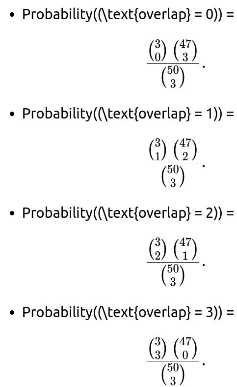
This completely characterizes the distribution of overlap. An interviewer may ask you to compute these probabilities explicitly and then verify they sum to 1. A pitfall occurs if you try to mix up the sample spaces (e.g., counting permutations or mixing up with-replacement vs. without-replacement) or forget to consider that once Alice’s set is fixed, Bob’s set must be chosen from the entire 50 as a combination of 3.

If the question extends to repeated picks over multiple rounds, how do we track the average overlap across time?

Sometimes, interviewers explore dynamic or repeated scenarios. Suppose Alice and Bob each pick 3 shows per “round,” for multiple rounds in a row. If each round is independent and the same selection process is used (uniformly at random from 50 shows), you can analyze each round identically and treat the total overlap as the sum of overlaps across all rounds.

The expected overlap in each round remains (\frac{9}{50}). Over (n) independent rounds, the expected total overlap is (n \times \frac{9}{50}). One might also be interested in how many times they have no overlap at all. By linearity of expectation, the expected number of zero-overlap occurrences out of (n) rounds is (n) multiplied by the probability of zero overlap (about 0.8273). For more advanced or realistic settings in which each new round depends on past picks (e.g., they cannot pick the same shows as before, or there is a memory-based preference), you’d need a Markov chain approach or a dynamic programming approach to capture how their sets evolve over time.

A subtle real-world scenario arises if each round’s choices are partly influenced by what was chosen previously, such as watchers switching shows if they’ve finished the previous ones. The distribution of picks in each round will then differ from the naive uniform assumption. Pitfalls include accidentally treating each round as independent when it truly isn’t, or ignoring the possibility that the available set might shrink or that personal preferences might shift over time.

If the question extends to more than two people, how do we compute the expected overlaps or probability of no overlap among three or more people?

Extending the same setup to three or more people (Alice, Bob, Carol, etc.) adds complexity to the computations. You might be asked for the probability that none of the three share any shows, or the expected number of common shows among all three, or pairwise overlaps.

One approach is to use multiple indicator variables. For instance, let (X_{i,j}) be the event that person (i) and person (j) share a particular show. Then use linearity of expectation to sum up the overlaps in pairwise fashion if you only need the expected total overlap across the group.

For the probability of zero overlap among all three, consider how:

• Alice picks 3 shows from 50.

• Bob must pick 3 from the remaining 47 for zero overlap with Alice.

• Carol then must pick 3 from the remaining 44 for zero overlap with both Alice and Bob if those two sets also had no overlap.

More precisely, the probability that all three sets of 3 are disjoint is

if each person’s selection is chosen from (\binom{50}{3}) possibilities independently. You can generalize for more people by continuing to reduce the available pool. Pitfalls occur in mixing up the step-by-step approach: you must carefully track how many shows are “used” by previous people to avoid counting impossible overlaps incorrectly. Also, if the order of picking doesn’t matter (i.e., all picks happen “simultaneously”), you still typically fix one person’s pick, then look at the conditional ways the others can pick disjoint sets, and finally normalize by the total ways everyone can pick.

If we want to approach bounding these probabilities with combinatorial bounds or inequalities like Markov’s inequality or Chernoff bounds, how might we do that?

Sometimes exact combinatorial expressions are cumbersome, especially in large-scale situations (for instance, if each person is picking a large subset out of an even bigger set). In those cases, bounding techniques are useful:

Markov’s inequality states that for a nonnegative random variable (X),

You can bound the probability that the overlap is large by applying Markov’s inequality. For example, if the expected overlap is (0.18), you can bound the probability that the overlap exceeds 1, or 2, etc. Chernoff bounds apply to sums of independent Bernoulli random variables, so if you approximate each show’s “common pick” indicator as a Bernoulli variable, you might apply Chernoff’s bound for large numbers of shows and picks, with the caution that picking 3 out of 50 introduces slight correlations.

These bounds are looser than exact combinatorial formulas, but in high-dimensional or large-scale settings, such approximations or bounds are valuable. A common pitfall is applying Chernoff bounds incorrectly when the picks are not truly independent or failing to interpret the bound’s limitations. In interviews, it’s important to clarify the assumptions under which these bounds hold to ensure the result remains valid.

If there is correlation between Alice’s and Bob’s picks, how does that change the analysis?

Real-world choices are seldom purely independent. If Alice and Bob influence each other’s picks (e.g., Bob is more likely to pick a show if he knows Alice enjoys it), the independence assumption breaks. To handle correlation, you need to specify a joint probability distribution for their choices.

The probability that both choose a particular show (i) is no longer (\frac{3}{50} \times \frac{3}{50}). Instead, it might be higher or lower depending on correlation. For instance, if Bob tends to emulate Alice’s preferences, the probability of overlap is higher than the independent case. One general approach is:

• Let (p_i) = Probability Alice picks show (i).

• Let (p_{i|A}) = Probability Bob picks show (i) given that Alice picked it.

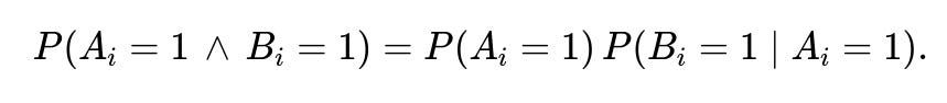
• Then the expected number of overlaps can be computed with indicator variables again, but each (E(X_i)) = (P(A_i = 1 ,\wedge, B_i = 1)). If you know the correlation structure, you can try to write

  

  When extended to sets of size 3, you must ensure the sum of picks remains 3 for each person while also respecting correlation constraints. This can become quite involved. A pitfall is to assume naive independence where it does not exist, or to incorporate correlation incorrectly (for instance, applying standard combinatorial formulas that require independence). In an interview setting, clarify how the correlation is defined so you can carefully account for it.

  If each show has a certain popularity that influences the picks (like a “weighted” random selection), how do we handle that?

  A more realistic scenario is that each show has a popularity or probability weight, and Alice or Bob is more likely to pick shows with higher popularity. One might model each person’s picks using a categorical distribution across the 50 shows, conditioned on the fact that exactly 3 distinct shows must be chosen. This is sometimes approached by:

  • Assigning weights (w_1, w_2, \dots, w_{50}).

  • Normalizing them so they sum to 1.

  • Drawing 3 distinct shows in proportion to these weights.

  The probability that a show (i) ends up in a person’s final selection is no longer uniform. To compute the probability that show (i) is picked, you would sum over all ways show (i) could appear in the 3 draws under the weighted distribution. For two correlated or uncorrelated pickers, you’d combine their respective probabilities or joint distributions.

  The expected overlap can still leverage indicator variables, but (E(X_i) = P(A_i=1)P(B_i=1)) only if independence holds in the selection of that show. If each person’s selection is independent but weighted, then

  

  But you must calculate (P(A_i=1)) and (P(B_i=1)) under the new weighting scheme. The probability of no overlap also becomes more challenging, as the combinatorial ratio approach is replaced by sums or integrals over the weighted subsets. A pitfall arises if you incorrectly use the uniform distribution formulas, ignoring that some shows might be far more likely to be chosen than others. In real-world recommender systems, popularity-based weighting often means common overlap is higher than uniform random selection would suggest, so the naive uniform results would underestimate overlap frequency.

  If we want to use this scenario in a machine learning or recommendation context, how might we design a model to predict how many shows two random viewers share?

  Although the original question is purely combinatorial, interviewers may bridge into machine learning. For instance, one could imagine a scenario where we want to predict the overlap in watch histories or top picks for two random users. Potential directions include:

  1. Probabilistic Modeling: A straightforward approach might use a parametric distribution (e.g., a Poisson-binomial or hypergeometric-based model) if we know how many items each user typically consumes and the popularity distribution of items.

  2. Collaborative Filtering: In real recommender systems, we might learn latent factors for each user and each show, then model the user’s likelihood to pick a particular show based on user–show affinity. The overlap between two users can be inferred by correlating these latent representations.

  3. Neural Architecture: If we have large-scale data about users’ watch habits, a deep learning model (e.g., a neural collaborative filtering architecture) could be trained to output the expected overlap or the probability that two users share a specific item. One might incorporate features such as demographic similarity or historical similarity in watch patterns.

  4. Practical Implementation Details: In large-scale systems, storing a full user–user overlap matrix is often infeasible. Instead, approximate techniques like locality-sensitive hashing or MinHash are used to estimate set overlaps quickly. Alternatively, random sampling methods or offline processing can produce approximate overlap statistics.

  A subtle pitfall in a real ML context is to conflate observed watch data (which might be partial or influenced by user interface constraints) with truly random picks. Another practical edge case is that certain highly popular shows might dominate the overlap, so naive models that assume uniform or independent picks might be systematically biased. In an interview, be prepared to discuss how you would handle cold-start users with little watch history or how you would incorporate time dynamics (users changing preferences) into your model.