
ML Interview Q Series: Using the SVM Kernel Trick to Learn Non-Linear Classification Boundaries.

📚 Browse the full ML Interview series here.
SVM and the Kernel Trick: Explain how Support Vector Machines can learn non-linear decision boundaries using the kernel trick. What is a kernel function and how does it allow an SVM to operate in a high-dimensional feature space without explicitly computing coordinates in that space? Provide an example of a commonly used kernel.
Understanding how Support Vector Machines (SVMs) can learn non-linear decision boundaries centers around the concept of mapping data to a high-dimensional (and sometimes infinite-dimensional) feature space, then finding a linear separating hyperplane there. Although it might appear computationally prohibitive to directly perform such a high-dimensional mapping, the kernel trick lets the SVM implicitly compute the inner products in this extended feature space, never explicitly constructing the coordinates. A kernel function is simply a function that, for any two input points in the original space, yields the inner product of their images in the transformed feature space.
Below is a comprehensive explanation covering how this works and why it is so powerful, followed by several potential follow-up questions that might arise in an interview and thorough discussions of the answers to each. The ideas and subtle points related to kernel choice, the mathematics behind SVM optimization, and real-world implementation considerations are also covered in depth.
SVMs are a fundamental technique in machine learning, particularly powerful when used with appropriate kernel functions. They rely on strong mathematical underpinnings that allow them to tackle both linearly separable and non-linearly separable problems effectively, often with robust generalization properties.
Deep exploration of these details in an interview setting, including potential pitfalls and edge cases, can set you apart and demonstrate both conceptual mastery and applied understanding.
Intuitive Overview of How SVMs Work
An SVM tries to find a decision boundary (hyperplane) that maximizes the margin between two classes (for binary classification). In cases where data is linearly separable, SVM searches for the widest gap that separates the classes without misclassification. However, data often cannot be separated by a simple linear boundary in the original space. To address this, the SVM can transform the data into a (usually) higher-dimensional space where it can be linearly separable, then find a linear hyperplane there.
The Concept of Feature Mapping
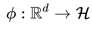
The key idea is to define a mapping function:
ϕ(x)
that transforms the original input vector (in, say, a space of dimension d) into a higher-dimensional (or even infinite-dimensional) space, usually denoted as a feature space. In that feature space, you could theoretically write:
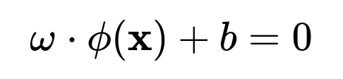
where (\mathcal{H}) is some high-dimensional Hilbert space (often referred to as the feature space). If the data become linearly separable in that transformed space, you can then construct a linear hyperplane in (\mathcal{H}):
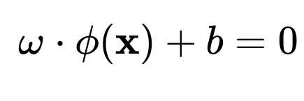
where (\omega) is the normal to the hyperplane in that high-dimensional space, and (b) is the bias term.
The Kernel Trick
Mapping data into a huge space might be extremely costly. If each data point in the original space (\mathbf{x}) has a dimension (d), transforming it via (\phi) into a very large or infinite dimension might appear computationally intractable. However, a kernel function:
k(x,z)
is defined such that it computes the inner product of two images in the feature space directly:
k(x,z)=ϕ(x)⋅ϕ(z)
But the crucial advantage is that you never need to explicitly compute (\phi(\mathbf{x})). Instead, you only need to be able to compute (k(\mathbf{x}, \mathbf{z})) for any pairs of points (\mathbf{x}) and (\mathbf{z}) in the original input space. This property dramatically reduces computation, because much of the SVM’s formulation in its dual representation relies on dot products between training examples. By replacing all (\phi(\mathbf{x}_i) \cdot \phi(\mathbf{x}_j)) with (k(\mathbf{x}_i, \mathbf{x}_j)), you effectively perform the linear classification in the high-dimensional space without ever working with the explicit high-dimensional coordinates.
Mathematical Formulation and Dual Representation (Brief Overview)
The SVM optimization often appears in two forms: the primal formulation (in terms of (\omega) and (b)) and the dual formulation (in terms of Lagrange multipliers (\alpha)). For classification, the dual form is critical in understanding the kernel trick because it expresses the decision function as a sum of kernels evaluated between the test example and the support vectors:
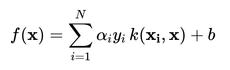
Here, (N) is the number of training examples, (\alpha_i) are the learned Lagrange multipliers, (y_i \in {-1, +1}) are the class labels, and (k(\mathbf{x_i}, \mathbf{x})) is the kernel function.
Because this formulation needs only (k(\mathbf{x_i}, \mathbf{x_j})) instead of explicitly calculating (\phi(\mathbf{x_i})) and (\phi(\mathbf{x_j})), the SVM “implicitly” operates in the high-dimensional space. This is the essence of the kernel trick.
Commonly Used Kernels
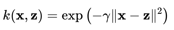
A kernel must satisfy Mercer’s condition, ensuring it corresponds to some valid (positive semi-definite) inner product in a Hilbert space. Many standard kernel functions have been developed and tested. One of the most commonly used is the Radial Basis Function (RBF), also known as the Gaussian kernel:
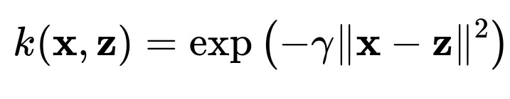
where (\gamma > 0) is a parameter that controls the width of the Gaussian influence. This kernel can map a single point in the original space to an infinite-dimensional Hilbert space, yet computations remain feasible because you only ever need the scalar value of (k(\mathbf{x}, \mathbf{z})).
In practice, SVM libraries (like the ones in scikit-learn, libSVM, and others) allow you to choose from various kernels, including polynomial, sigmoid, RBF, and even custom kernels you define (as long as the kernel is valid under Mercer’s condition).
Example Python Code Using an RBF Kernel
Below is a simple illustration of using scikit-learn’s SVM (with the RBF kernel) in Python:
from sklearn import svm
from sklearn.datasets import make_blobs
from sklearn.model_selection import train_test_split
from sklearn.metrics import accuracy_score

# Generate synthetic data
X, y = make_blobs(n_samples=200, centers=2, random_state=42, cluster_std=2.0)

# Split into training and testing
X_train, X_test, y_train, y_test = train_test_split(X, y, test_size=0.3, random_state=42)

# Create and train the SVM model with RBF kernel
model = svm.SVC(kernel='rbf', gamma='scale', C=1.0)
model.fit(X_train, y_train)

# Predict on test set
y_pred = model.predict(X_test)

# Calculate accuracy
accuracy = accuracy_score(y_test, y_pred)
print("Test set accuracy:", accuracy)
This snippet shows how easy it is to apply an SVM with the RBF kernel in practice. Under the hood, it is applying the kernel trick to separate the data in a higher-dimensional space.
Why Kernels Are Powerful in Non-Linear Settings
When data is not linearly separable in the original space, an SVM with a kernel tries to transform the representation via (\phi). The capacity to find a linear boundary in that transformed space allows the model to capture highly non-linear structures. In essence, the boundary in the original space becomes a non-linear curve (or manifold) that can separate classes effectively.
Potential Follow-Up Questions
Below are several in-depth follow-up questions that interviewers might ask, each with a comprehensive discussion of the answers and subtleties to watch out for.
What are the advantages of using the kernel trick compared to explicitly mapping into a higher-dimensional feature space?
One major advantage is computational efficiency. If you tried to construct, for instance, all polynomial feature combinations up to a certain degree, you might end up with combinatorial explosion in the number of features. By using the kernel trick, you only need to evaluate the kernel function (k(\mathbf{x_i}, \mathbf{x_j})) for pairs of data points without constructing these high-dimensional vectors.
Another advantage is the theoretical foundation provided by Mercer’s theorem, which ensures that if a kernel is positive semi-definite, it corresponds to some dot product in a (potentially) high or infinite-dimensional feature space. This allows SVMs to achieve significant flexibility in capturing complex decision boundaries while preserving generalization capabilities.
How do you choose which kernel to use?
In practice, the RBF (Gaussian) kernel is often the default choice because it works well in many situations without much feature engineering. However, the best kernel choice can be dataset-dependent. One might select a polynomial kernel if the data suggests polynomial-like boundaries or prior knowledge indicates polynomial relationships. A sigmoid kernel might be chosen if the data exhibits certain logistic-like boundaries.
Model selection often involves cross-validation to tune kernel-specific hyperparameters (like (\gamma) in the RBF kernel or the polynomial degree in a polynomial kernel), as well as the C parameter (soft-margin penalty) that controls the trade-off between margin size and classification error.
What is the role of the parameter (\gamma) in the RBF kernel and how does it impact model performance?
The parameter (\gamma) controls the width of the Gaussian in the RBF kernel:
If (\gamma) is too large, the Gaussian function becomes very peaked, making each training example have a very narrow region of influence. The model can become overly sensitive to individual data points, leading to potential overfitting. If (\gamma) is too small, the kernel decays more slowly, and the resulting decision boundaries might be too smooth to capture the complexity of the data, leading to underfitting.
A typical practice is to search for (\gamma) (and the penalty parameter C) through grid search or random search with cross-validation to find a good balance between bias and variance.
Could you provide an example of a polynomial kernel and discuss when you might use it?
Yes, a polynomial kernel might look like:

where (d) is the polynomial degree and (c) is a constant term. This kernel corresponds to all polynomial feature interactions of a certain degree (d). It might be used when you expect polynomial-like boundaries between classes or you suspect polynomial interactions among features. However, polynomial kernels can lead to high complexity for large degrees. Balancing the degree, the constant term, and SVM’s penalty parameter C is crucial. In many practical applications, the RBF kernel is still preferred due to its flexibility and smoothness, but the polynomial kernel can be very effective in certain domains (e.g., certain natural language processing tasks or in polynomial regression scenarios).
What is the computational complexity of an SVM using the kernel trick?
When using kernel methods, the training complexity can become more expensive for large datasets, as it often scales around (O(N^2)) or (O(N^3)) depending on the specific implementation, where (N) is the number of training points. The SVM training typically requires evaluating the kernel between pairs of training samples. For extremely large datasets, this can become prohibitive, and specialized approximate methods or linear SVMs (for large-scale linear problems) might be preferred. Various approximate kernel methods and random feature expansions have been developed to mitigate the cost, but the naive kernel SVM approach can be quite expensive for very large (N).
What happens if the kernel you pick does not satisfy the Mercer condition?
If a kernel is not positive semi-definite, it does not correspond to a valid inner product in any Hilbert space. In practice, many SVM libraries check for numerical issues during training or might fail to converge if the kernel matrix is not positive semi-definite. In general, you should use a known valid kernel function. If you design a custom kernel, verifying Mercer’s condition can be non-trivial, but it is critical for the SVM to function correctly.
What is the soft margin concept and how does it relate to kernels?
Real-world data can be noisy and might not be perfectly separable, even in high dimensions. The soft margin SVM introduces a slack variable mechanism that allows some points to be misclassified or within the margin boundaries, controlled by the penalty parameter C. A larger C punishes misclassifications more severely, leading to potentially narrower margins. A smaller C might allow more points to fall into or across the margin, leading to a broader margin but potentially higher misclassification. This soft margin approach can still be paired with kernels, giving a flexible framework for non-linear classification that can handle noisy data.
Can SVMs with the kernel trick be applied to regression problems as well?
Yes. Support Vector Regression (SVR) uses a similar idea, but instead of maximizing the margin between classes, it tries to fit a function within an epsilon (ε) deviation from the training data, minimizing the magnitude of the coefficients to achieve flatness. The kernel trick is equally applicable to SVR: you replace all dot products in higher-dimensional feature spaces with a kernel function. This yields a robust regression technique that can capture non-linear relationships.
How do you interpret or visualize the decision boundary when using non-linear kernels?
When using a non-linear kernel, the decision boundary in the original input space is non-linear and can be quite complicated. Direct visualization is easy if you have only two features (2D) or three features (3D); you can plot the decision boundary or contour lines. In higher dimensions, direct visualization becomes less intuitive. However, you might resort to dimensionality reduction or partial dependence plots to glean some insights. Understanding the shape of the boundary in high-dimensional settings is intrinsically difficult, but you can still visualize slices or projections of the decision surface.
What are some real-world pitfalls when training an SVM with a kernel?
One pitfall is choosing kernel parameters that lead to overfitting (e.g., (\gamma) too large in the RBF kernel, a polynomial degree too high in a polynomial kernel, or a C value that is too large). Overfitting can manifest as excellent training performance but poor generalization. Another pitfall can be memory and computational constraints. For large datasets, storing and computing the kernel matrix can be infeasible. Additionally, if data has very high dimensionality but is also extremely sparse, certain kernels can lead to suboptimal or unstable behavior. You need to ensure data is standardized or scaled appropriately (especially for kernels that rely on distances, like the RBF kernel). Failing to scale data can drastically affect performance and hamper convergence.
Summary
Support Vector Machines extend beyond linear separation through the kernel trick, allowing them to model complex, non-linear decision boundaries by implicitly mapping input data to high- or infinite-dimensional feature spaces. The kernel function replaces explicit feature transformation and dot product computation, maintaining reasonable efficiency while capturing rich non-linear relationships. The RBF kernel is a widely used choice, although polynomial kernels and others can be suitable for specific tasks. Selection of hyperparameters like (\gamma) in the RBF kernel and the penalty parameter C is essential to avoid overfitting or underfitting. Overall, the mathematical elegance and strong theoretical foundation of SVMs, combined with the practical kernel approach, continue to make them a significant tool in a wide range of classification and regression problems.
Additional Follow-Up Questions and Explanations
How does one implement a custom kernel in a typical library like scikit-learn, and what practical considerations are involved?
In scikit-learn, you can provide a “precomputed” kernel matrix or pass a custom kernel function to an SVC model by specifying kernel='precomputed' and then passing the Kernel matrix of shape ((N, N)) for your training data. You’d also need to do the same precomputation for test data. You must ensure your custom kernel is valid (i.e., symmetrical and positive semi-definite). This usually implies verifying the kernel using domain knowledge or ensuring it can be constructed from known valid kernels through operations that preserve positive definiteness.
Practically, watch out for numerical stability, especially if your kernel values become extremely large or extremely small. Good data preprocessing (such as scaling or normalizing inputs) is critical for custom kernels to behave well.
Could you discuss the role of the bias term (b) in the high-dimensional feature space?
In the primal form, the SVM tries to find a hyperplane:
When you move to the dual form, the bias (b) can be found by ensuring the Karush–Kuhn–Tucker (KKT) conditions hold for support vectors that lie on the margin. In practice, once the (\alpha_i) values are learned, you choose a support vector with (\alpha_i > 0) (and typically less than C if a soft margin is used) and solve for (b). In the dual representation:
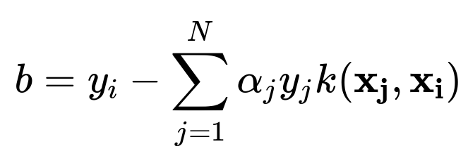
for any such support vector (\mathbf{x_i}). This ensures the correct offset in the final decision boundary equation. Conceptually, (b) acts as the shift that orients the hyperplane in the transformed space.
In practice, do we still need linear SVMs if kernel SVMs are more flexible?
Yes. Linear SVMs are extremely popular in large-scale and high-dimensional contexts (like text classification with millions of features). In such contexts, a kernel-based approach might be intractable due to memory and CPU constraints. Linear SVMs (often implemented with coordinate descent or dual coordinate descent) can train very fast on massive datasets, and often yield sufficiently good performance. Also, if the data is believed to be roughly linearly separable in its current representation, a linear SVM might be all that’s needed.
Below are additional follow-up questions
How can we extend kernel-based SVMs to multi-class classification scenarios, and what are the potential pitfalls?
Although the basic formulation of SVMs focuses on binary classification, they can be adapted to multi-class settings in several ways. Two common strategies are One-vs-Rest (OvR) and One-vs-One (OvO):
One-vs-Rest (OvR) Approach • Train a separate classifier for each class, treating that class as “positive” and all other classes as “negative.” • When predicting a new sample, all classifiers produce a decision score. The class whose classifier gives the highest score (or most confident margin) is chosen.
One-vs-One (OvO) Approach • Train separate classifiers for every pair of classes (for k classes, this yields k(k - 1)/2 classifiers). • During prediction, each classifier “votes” on which of the two classes the new sample belongs to. The class with the most votes wins.
Potential Pitfalls and Edge Cases • Scalability: OvO grows quadratically with the number of classes, which may become computationally expensive for large k. • Imbalanced Class Distribution: In heavily skewed multi-class data, some binary sub-problems might have very few samples of a particular class. This can lead to poorly calibrated decision boundaries. • Inconsistent Decisions in OvR: Different binary classifiers might all indicate “positive” or “negative” for a single sample, causing ambiguous or conflicting predictions. Proper calibration of decision scores can mitigate this confusion. • Kernel Selection: In multi-class scenarios, kernel hyperparameters might need to be tuned more carefully because the feature transformations must effectively separate multiple classes, not just two.
Can we train kernel SVMs incrementally or on streaming data, and what are the key challenges?
Traditional SVM implementations rely on a batch approach: you load the training data, compute the kernel matrix (partially or entirely), and solve the optimization problem. For streaming or continually arriving data, retraining from scratch each time can be prohibitively expensive. Incremental SVM methods attempt to update the model when new data comes in without rebuilding from zero.
Key Challenges • Memory Constraints: Maintaining a dynamic kernel matrix as new data arrives can become very large and unwieldy. • Model Updates: Adjusting the Lagrange multipliers and support vectors on the fly is complex. Approximate methods or frameworks like budgeted SVMs limit the number of support vectors to keep memory usage consistent. • Non-Stationary Data: In streaming contexts where data distributions evolve over time (concept drift), the learned boundaries must be updated or “forgotten” if older data becomes less relevant.
Pitfalls • Performance Degradation: Incremental updates might be approximate, potentially lowering performance relative to a full batch solution. • Design Complexity: Implementations can be significantly more complex compared to standard batch SVM tools, making them prone to errors if not rigorously tested.
How do kernel-based SVMs handle highly imbalanced datasets, and what special considerations apply?
In imbalanced classification, one class might have vastly more samples than another. Standard SVM training can bias the decision boundary toward the majority class.
Special Considerations • Class Weighting: Adjusting the penalty parameter C differently for minority and majority classes can help. Many SVM implementations (e.g., scikit-learn’s class_weight parameter) allow you to assign higher cost to misclassifying minority-class points. • Kernel Hyperparameter Tuning: For RBF kernels, tuning (\gamma) can be crucial in ensuring minority samples receive enough local influence in the feature space. • Data Preprocessing: Techniques like oversampling (e.g., SMOTE) or undersampling can be combined with SVM training to rebalance class representation.
Pitfalls • Overfitting on Minority Class: Overly aggressive class weighting or oversampling can lead to classification boundaries that favor the minority class at the expense of overall performance. • Evaluation Metrics: Relying on accuracy alone in an imbalanced scenario is misleading. Alternative metrics (precision, recall, F1-score, ROC AUC, etc.) become crucial.
How can we interpret a kernel-based SVM for model explainability, and what are the limitations?
Kernel SVMs do not yield simple, globally interpretable coefficients like linear models do, because the decision function involves a potentially complex mapping to a higher-dimensional space.
Interpretability Approaches • Local Surrogate Models: Methods such as LIME (Local Interpretable Model-agnostic Explanations) can approximate the local decision boundary near a point with a simpler model (e.g., linear). • Support Vector Inspection: Analyzing which training samples become support vectors might offer insight into critical regions of the feature space. • Feature Contributions (Partial Dependence): One can attempt to assess how changes in a single feature—while others are held constant—affect the SVM’s output.
Limitations • Complex Feature Spaces: With kernels like RBF, the transformation is infinite-dimensional, making direct feature-importance measures difficult to define rigorously. • Local vs. Global Explanation: Many techniques can only provide local approximations; fully understanding the global boundary can be challenging.
When comparing kernel-based SVMs to neural networks, what are key differences and pitfalls in deciding which to use?
Although both methods can handle non-linear decision boundaries, they differ in architecture, training, and interpretability:
Key Differences • Data Requirements: Neural networks often need large amounts of labeled data to outperform classical methods, whereas SVMs can be competitive with fewer samples and proper kernel choice. • Feature Engineering: Kernel SVMs rely on carefully chosen kernels, while neural networks can learn hierarchical features from raw data, especially in domains like images or text. • Computational Complexity: Kernel SVM training can scale poorly with large datasets, whereas neural networks can leverage GPUs and parallelism.
Pitfalls • Overfitting with Certain Kernels: If you incorrectly tune (\gamma) for the RBF kernel or the polynomial degree, an SVM might severely overfit. Neural networks also overfit without proper regularization or architecture choices. • Hardware and Framework Support: Modern deep learning frameworks (e.g., PyTorch, TensorFlow) are well-developed, while large-scale kernel-based solutions may be less readily available.
Beyond grid search, what advanced strategies exist for optimizing kernel hyperparameters, and what are potential pitfalls?
Advanced Strategies • Bayesian Optimization: Models the hyperparameter space as a function to be optimized. Uses a surrogate function (e.g., Gaussian Process) and an acquisition function to pick the next hyperparameter set. • Hyperband/Successive Halving: Allocates progressively more resources to promising hyperparameter configurations. • Genetic Algorithms: Uses evolutionary strategies to search a hyperparameter space.
Pitfalls • Computational Overheads: Bayesian optimization or genetic algorithms can become expensive if each evaluation involves full SVM training. • Local vs. Global Optima: Some methods might converge to local optima in high-dimensional hyperparameter spaces. Carefully designed search spaces can mitigate this. • Complex Interactions: Kernel hyperparameters can interact with the regularization parameter C in subtle ways; blindly optimizing one dimension without considering the other might yield suboptimal results.
Are there approximate methods to handle very large datasets with kernel SVMs, and what are the trade-offs?
Yes, several approximate or “low-rank” methods tackle the kernel computation bottleneck:
Random Fourier Features (RFF) • Concept: Approximates the RBF kernel by mapping data into a low-dimensional space using random Fourier basis. • Implementation: Replace the kernel function with an explicit feature map (\tilde{\phi}(\mathbf{x})). Then train a linear model in that space. • Pitfalls: Approximation error depends on the dimension of the random feature map. If the dimension is too small, the approximation might degrade accuracy.
Nyström Method • Concept: Use a subset of data (landmark points) to approximate the kernel matrix, reducing computational cost. • Pitfalls: Choice of subset (and subset size) critically impacts performance. A poor subset might yield a suboptimal approximation.
Trade-offs • Memory Usage: Approximate methods can drastically reduce memory footprint for large N. • Accuracy vs. Speed: Achieving near-exact kernel behavior might require sufficiently large expansions or subsets, partially offsetting computational savings.
How does missing data or noisy features impact kernel SVM performance, and what steps can be taken to mitigate issues?
Kernel SVMs depend on accurate distance or inner product estimates among samples. Missing data or highly noisy features can distort these distances.
Mitigation Strategies • Imputation: Techniques like mean imputation, K-nearest neighbors imputation, or model-based approaches. However, poor imputation can introduce bias in the kernel space. • Feature Selection or Dimensionality Reduction: Removing or reducing the impact of noisy features can stabilize distance-based calculations. • Robust Kernels: In domains like computer vision, specialized kernels that incorporate robust distance metrics (e.g., histogram intersection kernels) can reduce sensitivity to noise or partial data.
Pitfalls • Correlation with Labels: If the missingness is not random (i.e., data is missing systematically related to the label), naive imputation can bias the SVM boundary. • Complex Hyperparameter Interactions: Even after imputation, the kernel hyperparameters (like (\gamma)) might need re-tuning to handle altered distances effectively.