
ML Interview Q Series: Valuing First-Mover Advantage in a Dice Game Using Probability and Expected Value
Browse all the Probability Interview Questions here.
15. A and B are playing the following game: a number k from 1–6 is chosen, and A and B will toss a die until the first person sees side k. That person then gets $100. How much is A willing to pay to play first?
This problem was asked by Lyft.
Below is an extremely thorough and in-depth explanation, structured under various headings and subheadings. It addresses how to derive the exact probability that player A (the first to roll) will be the winner, explains the necessary mathematics, and answers a series of anticipated follow-up questions in a typical tough FANG interview environment. It also explores practical nuances and hidden pitfalls that might come up in real interviews.
All Latex is wrapped as requested (either inline with "$" or centered in H1 style with
# $$ your expression here $$
). Python code examples are wrapped in triple backticks ```py as requested. No lists are numbered.
Intuitive Overview of the Game
Player A and Player B each want to be the first to roll a specific side, k, on a fair six-sided die. The game proceeds in turns:
A rolls first.
If A gets side k, A wins $100 immediately and the game ends.
If not, B rolls next.
If B gets side k, B wins $100 immediately and the game ends.
If neither sees side k, the turns alternate indefinitely until side k appears for the first time.
Because A rolls first, A has an inherent advantage. We want to quantify exactly how big this advantage is. That advantage, when converted to an expected monetary value, tells us how much A should be willing to pay for the privilege of going first.
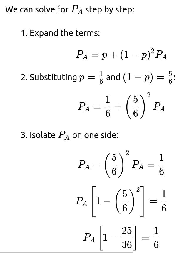
Probability that A Wins When Rolling First
Core Mathematical Reasoning
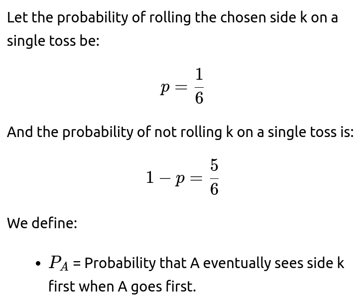
On A’s very first roll:
With probability p, A succeeds immediately and wins the $100 right away.
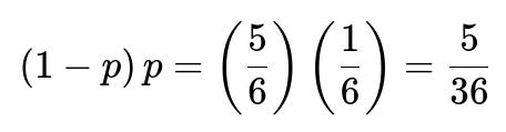
With probability (1−p), A does not see side k on that first roll, and then B gets a chance to roll.
When B rolls (assuming A failed), B can also succeed with probability p. If B succeeds, B wins, and A loses. That scenario happens with probability:


Expected Value for Player A Going First
Since the payout is $100 to the winner, the expected monetary return for A, going first, is:

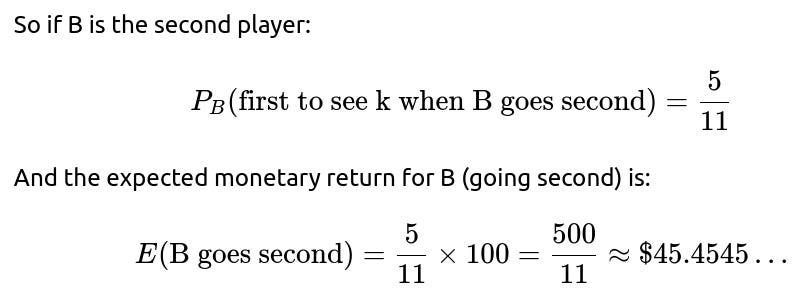
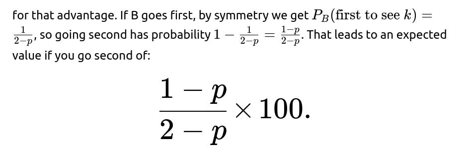
Expected Value for Player B if A Goes First
Given that A has probability 6/11 to be the first to roll k, B must have probability 5/11 (the probabilities must sum to 1, ignoring the impossibility of an infinite loop without success, since eventually the side k should appear).
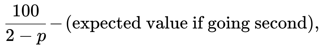
How Much is Going First Worth?
If you are A, you can either go first or let B go first. The advantage is the difference in your expected payoff.
Going first: $54.5454...
Going second: $45.4545...
The difference is:
54.5454…−45.4545…=9.0909…
In exact fractional form:
So A should be willing to pay up to about $9.09 (repeating) for the right to go first.
Alternative Derivation (Geometric Summation)


Practical Python Simulation
You can confirm this with a quick Monte Carlo simulation in Python. This simulation can be used in an interview to illustrate that you not only understand the math but also how to verify it empirically.
import random

def simulate_games(num_games=10_000_000):
    import math
    wins_for_A = 0
    for _ in range(num_games):
        # We assume the chosen side is k = 1 (it doesn't matter, symmetrical)
        # A goes first
        while True:
            # A's roll
            roll = random.randint(1, 6)
            if roll == 1:
                wins_for_A += 1
                break
            # B's roll
            roll = random.randint(1, 6)
            if roll == 1:
                break
    return wins_for_A / num_games

if __name__ == "__main__":
    prob_A_wins = simulate_games()
    print("Estimated Probability A Wins:", prob_A_wins)
Over a large number of runs, the proportion of times A wins will hover very close to 6/11 (about 0.5454545...).
Subtle Points and Potential Pitfalls
One might be tempted to think the advantage is larger because going first often “feels” more powerful. In reality, the difference in expected value is roughly $9.09 out of $100. Some interviewees mistakenly guess a more significant advantage like $20 or $30.
A potential pitfall is to assume the probability that A wins on a given cycle is p/(p+p) or something simplistic. The correct approach must account for the possibility that both fail, leading to repeated cycles.
Another subtlety is that the die eventually will show side k, so there is a 100% chance the game ends. This ensures the geometric series or the recursion approach is valid.
Potential Real-World or Variation Scenarios
Some FANG-style interviews might expand this puzzle to test broader comprehension:
What if the die is biased?
What if instead of a 6-sided die, we have an n-sided die or an unknown distribution?
How does this generalize to more than two players?
These follow-up questions probe your deeper understanding of Markov chains, geometric distributions, and how to handle different probabilities of success per turn. Often, the logic of “first success in repeated Bernoulli trials with multiple participants” is an entry point into more advanced probability modeling.
Follow-up Question: “What if the die is biased, with probability p of rolling side k, instead of 1/6?”
When the die is biased, we still define p as the probability that the chosen side k appears on any single roll. The entire approach generalizes neatly:


A might pay up to
Hence, the difference is:

In the fair-die scenario where p=1/6, that difference simplifies to:

consistent with the earlier result.
Follow-up Question: “Could this be approached with a Markov chain formalism?”
Yes. We can create a Markov chain with states that represent whose turn it is and whether the game has ended. However, since the game terminates as soon as k appears, we can simplify to states representing (A’s turn, B’s turn) with an absorbing state if k is seen. In this chain:
From state (A’s turn), with probability p, you go to an absorbing state (A wins). With probability (1−p), you move to (B’s turn).
From state (B’s turn), with probability p, you go to an absorbing state (B wins). With probability (1−p) you go back to (A’s turn).

Follow-up Question: “How do we implement a quick check for the difference in expected value in code?”
If an interviewer asks for the difference in expected payoffs, we can code it directly:
def expected_value_difference_fair_die():
    p = 1/6
    # Probability A wins going first
    pA = 6/11  # or derived from the recursion
    # Probability A wins going second is the complement (since if A doesn't go first, B has that advantage)
    pA_second = 5/11

    # A's expected value going first
    EV_A_first = pA * 100
    # A's expected value going second
    EV_A_second = pA_second * 100

    difference = EV_A_first - EV_A_second
    return EV_A_first, EV_A_second, difference

if __name__ == "__main__":
    ev_first, ev_second, diff = expected_value_difference_fair_die()
    print("A's EV going first:", ev_first)
    print("A's EV going second:", ev_second)
    print("Difference (what A would pay):", diff)
Running it (or just doing the math) confirms the difference is $9.09 repeating.
Follow-up Question: “What if we had multiple dice, or multiple chosen sides?”
Interviewers might see if you can extend the logic to more complicated scenarios. For example, imagine that each turn you roll two dice at once, and you’re looking for side k on either die. The probability of success in one turn for that player becomes:

Follow-up Question: “Are there any practical real-world applications of this puzzle concept?”
Yes. This puzzle is a simplified demonstration of:
Geometric random variables.
Bernoulli processes where multiple players race to the first success.
“First to success” auctions or scenarios in competitive bidding, where each participant takes turns, paying a cost each turn, until an event of interest occurs.
In game theory or e-commerce (like bidding or random events in computer systems), the principle of how valuable it is to go first in a repeated trial setting can be crucial.
Concluding Remarks on the Worth of Going First
Putting it all together, for a single fair 6-sided die and a single target face k, the first mover’s probability of eventually seeing k first is 6/11. That yields an expected value of about $54.55, compared to $45.45 for the second mover. The advantage of going first is $9.09, meaning A should be willing to pay around $9.09 to be the one who rolls first.


Below are additional follow-up questions
If the game was changed so that the target side k is decided randomly after each roll, how would that affect the advantage for going first?
In this new variant, the chosen side k is not fixed throughout the entire game. Instead, after each roll (whether by A or B), a new side k is randomly chosen from 1–6 with equal probability. This means that before each new roll, the “winning” condition can suddenly shift to a different side.
Detailed Explanation and Logical Steps:
Imagine A rolls first. In each turn, the target might be 1 for the first roll, then (if missed) it might become 3 for the second roll, then 5 for the third, and so on—each time newly and independently chosen from the six sides. The main subtlety is that on each player’s roll, we do not just have a fixed success probability of 1/6 for the same side. Instead, it’s always 1/6 that the outcome matches the newly chosen target side.
A still gets the very first attempt to match the (newly decided) target side k. So on roll #1, A has probability 1/6 to succeed immediately.
If A fails (with probability 5/6), then B rolls. However, the target changes again right before B’s roll. B now has a 1/6 chance to match the newly chosen side and win on that second roll.
If B also fails (probability 5/6 on B’s attempt), the turn passes back to A, and once again the side is re-chosen at random. This cycle continues indefinitely.
The crucial difference from the original scenario is that each roll has a “fresh” target side chosen with probability 1/6 of success, decoupled from the prior roll. However, from a purely probabilistic standpoint, each roll is still “one Bernoulli trial with success probability 1/6.” It turns out the essential advantage from going first remains the same: each cycle (consisting of one roll by A and then one roll by B if A fails) is effectively:
A tries first with probability 1/6 to succeed on that roll.
If A fails (5/6 chance), B tries with probability 1/6 to succeed on his roll.
Thus, the same geometric recursion logic applies. After both fail, we are “back to square one,” with A to roll again under the same situation. So the probability that A eventually wins is still 6/11, and the advantage is still $9.09.
Potential Pitfalls and Edge Cases:
Someone might incorrectly assume that changing the target side more frequently influences the advantage, but since each roll is always 1/6 chance to succeed, the structure remains a straightforward “I roll first, you roll second” with a repeated cycle until success.
An edge case would be if the random choice of k were skewed (e.g., certain sides are more likely to be chosen), or if the next choice of side depends on previous rolls. That would require a more customized analysis.
If the random re-selection happens only occasionally (rather than after every single roll), you’d need to adapt the probability of success per turn. But in the scenario described—fully random each roll—the advantage does not change from the standard game.
Hence, from an expected value standpoint, A’s advantage remains the same.
If we only allow a limited total number of rolls, how does this change the advantage for going first?
In a practical scenario, the players might say: “We will roll at most N times. If no one gets side k within N rolls, the game ends in a draw (no one wins).” This changes the analysis significantly, because the game is no longer guaranteed to end with a winner.
Detailed Explanation and Logical Steps:
Let N be the maximum number of total die rolls across both players. A rolls first, then B, and so on, until either a winner is found or we have used up N rolls.
We can compute the probability of A winning by enumerating cases or using a finite Markov chain:
A can win on roll 1 (probability 1/6).
If A misses, B has a chance to roll on roll 2. If B also misses, we go to roll 3 for A, etc.
The difference is that we must stop once we’ve used up N rolls.
If neither has succeeded by the time we reach the N-th roll, and that roll also fails to show side k, the outcome is a draw (nobody gets the $100).

We can explicitly compute A’s probability of winning by summing the probabilities that A succeeds on roll 1, or roll 3, or roll 5, etc., provided those rolls are ≤ N. We also must account for the possibility that B could succeed on any even-numbered roll ≤ N. If no success occurs by roll N, the game is a draw, so the total probabilities of (A wins + B wins + draw) = 1.
Typically, A’s advantage is even more pronounced for small N, because A might have strictly more rolls in total if N is odd. If N is large, the advantage tends to approach the infinite-roll limit of 6/11, but there’s always a possibility of a draw capping the game, which reduces the expected value for both players somewhat.
Potential Pitfalls and Edge Cases:
If N = 1, only A gets to roll. A’s probability of winning is 1/6, and B never even gets a turn. That drastically changes the advantage.
For small N, the advantage can be computed exactly using finite sums, but some might incorrectly apply infinite-series logic.
If the payout is split or there’s some other arrangement in the event of a draw, the payoff structure changes.
Hence, with limited rolls, you must handle the possibility of no one winning, which shrinks the expected payoff but typically preserves or even enhances the fraction of advantage for the first roller, depending on how N is set.
If the chosen side k is only revealed to Player A but not to Player B, what would happen?
In a scenario where A alone knows which side is the winning side, while B does not, you might wonder if A could exploit that knowledge somehow to gain a higher probability of success.
Detailed Explanation and Logical Steps:
Each player is physically rolling the same fair die, but B does not know which side they are aiming for. However, it’s still a fair 1/6 chance on any given roll that the hidden side appears.
The immediate question is: can A meaningfully take advantage of that hidden information? In a straightforward interpretation, not really. Because when A (or B) throws the die, the probability that the next toss is k is 1/6, regardless of whether the player knows that side.
A might attempt psychological tricks or to bluff B about which side is needed, but mathematically, each roll is unaffected by that knowledge. The moment A sees their success (roll matches k), the game ends. B doesn’t need to know the side to have the same 1/6 chance each roll.
The only scenario where hidden information might matter is if the players are allowed to do something like deliberately sabotage or re-roll. But if the rules require you to accept the roll’s result, knowledge of k does not change the underlying probabilities that cause the game to end.
Potential Pitfalls and Edge Cases:
Some might think that B’s ignorance drastically reduces B’s chances. In reality, each time B rolls, the probability is still 1/6 that the roll is k (the unknown side). B just doesn’t know which side it is, but physically, the random event is the same.
If the game had a strategy component—e.g., the ability to choose whether to “keep” or “reject” a roll, or place bets on certain outcomes—knowledge might help A. But in the basic “roll a fair die exactly once per turn and see if it’s k” game, hidden information does not create a strategic difference in the probability of success.
Hence, the fundamental 6/11 probability advantage for going first remains unchanged. The knowledge of k does not directly affect the mechanical probability of rolling that side for B.
What if players roll simultaneously on each turn? Would that change the advantage for going first?
In a version where A and B roll at the same time in each “round,” and we see who got k first in that same round, the outcome changes drastically.
Detailed Explanation and Logical Steps:
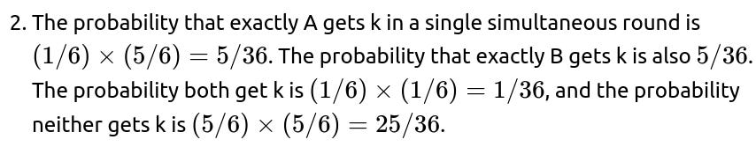
Under simultaneous rolling, define each round as:
Both A and B roll a die at the same moment.
If exactly one of them gets side k, that player wins immediately.
If both get side k simultaneously, perhaps we have a tie or a special tie-breaking rule (depending on the game’s definition).
If neither gets k, they proceed to the next round, rolling again simultaneously.

If the rule says that if they both get k in the same round, they re-roll or they share the prize, the advantage for going “first” disappears, because there is no concept of “first” in simultaneous rolling. They either keep rolling simultaneously or adopt a tie-breaker that might be symmetrical.
As a result, if both continue until exactly one sees k, you can compute the probabilities. But no single player gets the advantage of an earlier roll.
Hence, going first no longer confers the typical advantage seen in sequential play. The advantage might vanish entirely (or be replaced by a symmetrical probability of success if there is a tie-break rule).
Potential Pitfalls and Edge Cases:
Some might incorrectly apply the 6/11 logic to simultaneous rolls. That logic only applies if players roll sequentially.
If a tie in a round is broken by flipping a coin, then each is effectively 50–50 in that tie scenario, again erasing any advantage from “turn order.”
If the game stops as soon as both get k (and both share the prize), it leads to a different payoff structure. One must be careful in enumerating all possible outcomes.
Thus, in truly simultaneous rolling, the advantage of going first is nullified.
If there is a cost for each roll, how would that affect the amount A is willing to pay to go first?
Sometimes, each die roll might cost a small fee or each player might have to pay a certain cost per turn. This modifies the expected payoff analysis.
Detailed Explanation and Logical Steps:
Suppose each player must pay c dollars every time they roll the die. The winner still gets $100, but the net profit for each player depends on how many times they rolled before succeeding.

Probability that the game ends on the first roll (A’s roll) is p. In that scenario, A pays c once.
If it goes to B, we add an expected cost for B’s roll, then if both fail, we repeat. By carefully summing or using a Markov chain approach, we can find the average count of rolls for each.
If c is small relative to $100, A’s advantage in net payoff remains positive. If c is extremely large, there might be scenarios where going second is actually better because B might pay less in repeated attempts, making B’s net payoff occasionally higher. You have to do the full expected-value calculation to see the break-even point.
Potential Pitfalls and Edge Cases:
Some might ignore the cost distribution across players and just subtract the total cost from $100. But that’s incorrect. The costs are not paid equally if one player ends up rolling more times.
If the cost c is higher than the expected profit difference, it might invert who benefits from rolling first.
Hence, the cost factor can shrink or even negate A’s advantage, depending on how large c is relative to the incremental probability of winning.
What if the game could end with no winner if certain “lose” sides appear, or if multiple rolls pass without seeing side k?
Sometimes, variations impose a forced “loss” or forced stop. For example, if side 6 appears X times, the game ends for both players with no winner, or after M consecutive fails, they stop and no one wins.
Detailed Explanation and Logical Steps:
If certain outcomes terminate the game without awarding the $100, it changes the total probability mass that leads to a winner. Thus, the sum of probabilities “A wins” + “B wins” + “no winner” = 1.
The advantage of going first is still tied to the fraction of the time that a winner emerges. If the probability that the game ends with no winner is significant, then you must weigh how that might reduce the overall expected payoff for each player.
A common pitfall is to think “the advantage remains exactly the same.” Actually, the advantage could be diminished because if the game ends too early from a “lose condition,” neither player might get a robust second chance.
In general, you’d incorporate these new termination conditions into your states and compute the probabilities via a Markov chain or enumerating scenarios for how the game can progress. A can still have a “first mover advantage,” but the presence of possible forced termination can reduce the overall expected payoff for both and might shift the advantage fraction.
Hence, the presence of an additional “no winner” termination path means the advantage is typically smaller in absolute dollar terms, though the ratio of A’s winning probability to B’s winning probability might remain above 1.
How does this logic extend if there are three or more players, each rolling in sequence for side k?
If we generalize beyond just A and B, the dynamic changes further:
Detailed Explanation and Logical Steps:

Each player’s advantage depends on their order. Generally, the earliest players in the sequence have a higher probability of winning. A is the most favored, followed by B, and so on.


Potential Pitfalls and Edge Cases:
Some might incorrectly assume A always has the same advantage as in the two-player game. In reality, B and C are each behind A in the turn order, so their probabilities become smaller in proportion.
If you use a naive formula or only consider pairs, you must systematically handle all possibilities across the entire triple cycle.
If the game extends to four or more players, we can keep building the equations or use a Markov chain approach with states “Who is about to roll?” and keep track of transitions.
Thus, in multi-player expansions, the same conceptual approach works, but the algebra is more involved, and each subsequent player in the order has a lower chance of being the first to see k.
How would we handle a scenario where the probability of success p changes after each roll?
Sometimes, the event of interest might become more or less likely after each failure, or based on external conditions. For instance, after each unsuccessful roll, we might say “the next roll is more likely to see k” or “less likely,” or “p changes by some factor.”
Detailed Explanation and Logical Steps:

We calculate the probability that A eventually wins by summing transitions or by solving a system of linear equations for the absorbing states.
Generally, if the success probability tends to grow over time, the advantage of going first might be smaller if the highest probabilities occur in later rolls, which might be more accessible to B. Conversely, if success probabilities shrink over time, being first is more valuable because you get a higher initial p than B might get in subsequent rolls.
Potential Pitfalls and Edge Cases:
Failing to realize that the standard 6/11 logic does not hold if p is not constant from roll to roll.
Trying to use the same recursion formula but incorrectly substituting different values of p in each iteration. Instead, you need a more direct step-by-step or Markov chain approach.
Hence, the advantage can shift significantly based on how p changes across rolls. You must carefully define or measure the dynamic behavior of p.
If we incorporate a side bet that the losing player pays an additional $X penalty, does that alter how much A should pay to go first?
Sometimes games have side conditions. Suppose the first to roll k gets $100, but the loser must pay the winner an extra $X, or must pay the house $X.
Detailed Explanation and Logical Steps:
With an added penalty or side bet, the total swing in outcome can exceed $100. If the losing side must pay the winner $X, the winner effectively gains $100 + $X, while the loser is down $X. The game’s expected payoff for each player changes accordingly.
The advantage for A going first can be recalculated by:
Probability that A wins times the net gain for A if that happens
Probability that B wins times the net cost to A in that scenario

Potential Pitfalls and Edge Cases:
You might forget that a side bet changes the game’s payoff structure. Some might simply add $X to $100 for the winner without factoring in that this is paid by the loser, effectively doubling the advantage difference.
If the side bet is paid to a third party (the house) only by the loser, then the winner’s payoff might not include that side bet. Clarifying who pays and who receives is crucial.
Hence, side bets or additional penalties can change the value that a player might be willing to pay for first roll, but the underlying probability advantage is still the same 6/11 unless the side bet also influences how the game is played.
How do we ensure fairness if the die or environment might be tampered with?
In real-world contexts (casinos, gaming apps, etc.), there can be cheating or rigging that affects the fairness of the die rolls.
Detailed Explanation and Logical Steps:
If the die is not fair, the probabilities might deviate from 1/6, or be different for each roll. We must identify the actual distribution of outcomes to compute the advantage accurately.
If one player can manipulate the die (e.g., through weighting, controlled throws, or algorithmic tampering in a digital environment), the fundamental assumption that p=1/6 for the target side breaks down.
The advantage for going first can skyrocket or vanish altogether if, for example, the first player has a technique to ensure side k is more likely. Alternatively, if the environment is rigged such that the second roll is always more likely to show k, the advantage flips.
In practical, regulated settings, measures like randomization audits or cryptographic hashing can ensure that each roll is truly fair. If tampering is suspected, the entire analysis is moot, because the probabilities are no longer the standard 1/6.
Potential Pitfalls and Edge Cases:
Some might assume that a small deviation from 1/6 is negligible, but over many rolls it can drastically change the advantage.
If only A can exploit the tampered die, then A might have a much bigger advantage than the theoretical 6/11.
In digital contexts, pseudo-random number generators must be validated to avoid hidden biases.
Hence, in a tampered or uncertain environment, you must carefully measure or estimate the real probability distribution for each roll rather than assume ideal fairness.
How could we integrate a continuous-time viewpoint if the dice are rolled at arbitrary times rather than in discrete turns?
Some interviewers might push the concept further: in a continuous-time scenario, maybe A can roll any time they want, and then B can decide to roll at some different time, and so forth. This is less of a standard puzzle but might appear in real-time strategy contexts.
Detailed Explanation and Logical Steps:
If the rules are that each player can roll whenever they choose, we add an element of timing strategy: does A want to roll immediately, or wait? In standard discrete puzzles, A must roll first, then B rolls second. But in a continuous-time version, you can imagine each player choosing a time to roll.
Typically, if the event is memoryless (like a Poisson process), the advantage for going “first in time” can be considered. But if a game is truly continuous-time, players might race to roll as quickly as possible, removing any meaningful difference except who physically can act faster.
This extension can become quite complex, akin to auction theory in continuous time, where each player tries to be the first to do an action. The advantage might become purely about reaction speed and not about discrete turn orders.
Potential Pitfalls and Edge Cases:
Trying to treat a continuous-time scenario as if it’s still “A goes first, B goes second” can lead to confusion.
If there’s a cost to rolling over time or a limitation on how frequently you can roll, the analysis becomes a game-theoretic problem with dynamic strategy.
Hence, the simpler puzzle breaks down in a continuous-time environment. The standard 6/11 advantage is specifically about discrete turn-taking, not free-form rolling.
How do real casino games or random processes in online gambling confirm such theoretical probabilities?
In regulated real-world gambling or online platforms, the outcomes typically align with well-known probability laws. Operators must demonstrate the fairness of their random number generation so the house edge is consistent and known to players.
Detailed Explanation and Logical Steps:
Typically, a game with a “roll a die until event k occurs” structure is quite transparent. Audits can confirm that each side is equally likely.
Some online platforms provide a “provably fair” mechanism where the code or a cryptographic seed is made visible. Then players can verify the random draws are not manipulated mid-game.
The 6/11 advantage for the first mover is a fundamental outcome in a fair environment. If players suspect they are not seeing the expected distribution of wins, they might investigate potential tampering.
Real casinos might not offer a direct “race to see a single side” game in this simplistic form, but similar “first to roll a certain sum” or “beat the dealer by hitting a certain target” exist. The concept of sequential advantage or disadvantage is embedded in those rules (e.g., in Blackjack, the dealer acts last, which confers an advantage to the house).
Potential Pitfalls and Edge Cases:
Players might suspect the operator of rigging if the empirical frequency of the first player’s success is not near 54.545% over many trials. Small sample fluctuations are inevitable, but large persistent deviations could indicate a fairness issue.
Some might incorrectly attribute short-run variance to a fundamental shift in probability. Over many rolls, the law of large numbers should confirm that the first player wins about 6/11 of the time.
Hence, the theoretical advantage is well understood, and in properly regulated environments it can be validated empirically over large sample sizes.
