
ML Interview Q Series: What are some differences between the Undercomplete Autoencoder and the Sparse Autoencoder?


📚 Browse the full ML Interview series here.
Comprehensive Explanation
Undercomplete and Sparse Autoencoders are two distinct architectural or regularization choices for autoencoders that aim to learn compact representations of data. Both variants share the same essential structure: an encoder that transforms the input into a latent representation and a decoder that reconstructs the input from that latent space. The main difference lies in how each approach constrains the learned representations.
Undercomplete Autoencoder
An Undercomplete Autoencoder has a bottleneck layer with a smaller dimensionality than the input. By forcing the network to learn a compressed version of the data, it captures the most salient features necessary to reconstruct the original input.
It relies on the network’s inherent capacity constraints (a narrow bottleneck) and a suitable loss function, such as a mean squared error reconstruction loss or cross-entropy reconstruction loss. Because the hidden layer is smaller than the input dimension, the encoder is compelled to learn those compressed features that are most representative. If the network capacity is too high or the latent dimension is too large, an autoencoder might simply learn the identity function and fail to produce a meaningful compression. Undercompletion helps mitigate this risk.
Sparse Autoencoder
A Sparse Autoencoder can have an equal or even larger number of hidden units than the input. Instead of restricting the architecture by strictly reducing the number of neurons in the bottleneck layer, it imposes sparsity constraints on the hidden units. Most neurons in the hidden layer are encouraged to remain inactive (near zero activation) for a given input, which effectively forces the network to learn a sparse representation.
One common method is to use a sparsity penalty term that penalizes deviations from a target average activation. A typical penalty involves the Kullback-Leibler (KL) divergence between the average activation of each hidden neuron and a small fixed value that represents the desired sparsity.
Below is a representative formula for the loss in a Sparse Autoencoder with a reconstruction term plus a sparsity penalty.
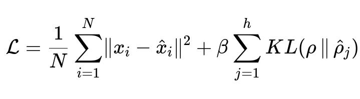
Here:
N is the number of training samples.
x_{i} is the original input for the i-th sample (dimension d).
\hat{x}_{i} is the reconstructed output for the i-th sample (dimension d).
h is the number of hidden neurons in the relevant hidden layer.
\rho is the sparsity parameter that defines the desired average activation for each hidden neuron.
\hat{\rho}_{j} is the empirically measured average activation of hidden neuron j across the dataset.
KL(\rho || \hat{\rho}{j}) is the Kullback-Leibler divergence between \rho and \hat{\rho}{j}, which grows larger when the average activation \hat{\rho}_{j} deviates significantly from the target \rho.
\beta is a hyperparameter that controls the contribution of the sparsity penalty relative to the reconstruction error.
In this way, the Sparse Autoencoder does not necessarily need a narrower bottleneck, but it imposes that each hidden neuron is active only for some subset of the inputs, achieving a form of capacity control that encourages robust and discriminative representations.
Key Differences
Undercomplete Autoencoder reduces the dimensionality of the hidden layer explicitly. Its fundamental constraint is architectural: fewer hidden units than input dimensions. This is a direct approach when the data is expected to have a low-dimensional manifold or a compressed underlying representation.
Sparse Autoencoder can have a hidden layer dimension greater or equal to the input dimension, yet it enforces a constraint through an additional sparsity penalty term. This means it controls capacity by forcing most neurons to be inactive for a given input. The representation it learns is not merely compressed by dimensionality but by encouraging most hidden units to remain zero (or close to zero) activation.
In practical scenarios, the Undercomplete approach is more straightforward when a known, smaller dimension effectively captures relevant features. The Sparse approach is more flexible and can uncover intricate and interpretable feature detectors (e.g., in image-based tasks, hidden units might learn Gabor-like filters), but it requires careful tuning of the sparsity hyperparameters.
Practical Example in Python
Below is a minimal illustration of how one might define and train both an Undercomplete and a Sparse Autoencoder in PyTorch. Note that for the Sparse Autoencoder, a KL divergence-like penalty or other sparsity penalty is applied to the average activation of hidden neurons.
import torch
import torch.nn as nn
import torch.optim as optim

# Dummy dataset
X = torch.randn((1000, 784))  # e.g., 1000 samples of 784-d input

# Undercomplete Autoencoder
class UndercompleteAE(nn.Module):
    def __init__(self, input_dim=784, hidden_dim=32):
        super(UndercompleteAE, self).__init__()
        self.encoder = nn.Sequential(
            nn.Linear(input_dim, hidden_dim),
            nn.ReLU()
        )
        self.decoder = nn.Sequential(
            nn.Linear(hidden_dim, input_dim),
            nn.Sigmoid()  # if data is normalized between [0,1]
        )

    def forward(self, x):
        z = self.encoder(x)
        x_recon = self.decoder(z)
        return x_recon

undercomplete_ae = UndercompleteAE()
optimizer = optim.Adam(undercomplete_ae.parameters(), lr=1e-3)
criterion = nn.MSELoss()

for epoch in range(5):
    optimizer.zero_grad()
    reconstruction = undercomplete_ae(X)
    loss = criterion(reconstruction, X)
    loss.backward()
    optimizer.step()
    # print("Epoch:", epoch, "Loss:", loss.item())

# Sparse Autoencoder (simple version)
class SparseAE(nn.Module):
    def __init__(self, input_dim=784, hidden_dim=256, sparsity_param=0.05, beta=1.0):
        super(SparseAE, self).__init__()
        self.sparsity_param = sparsity_param
        self.beta = beta

        self.encoder = nn.Sequential(
            nn.Linear(input_dim, hidden_dim),
            nn.ReLU()
        )
        self.decoder = nn.Sequential(
            nn.Linear(hidden_dim, input_dim),
            nn.Sigmoid()
        )

    def forward(self, x):
        z = self.encoder(x)
        x_recon = self.decoder(z)
        return x_recon, z

    def kl_divergence(self, rho, rho_hat):
        # element-wise KL
        return rho * torch.log(rho / (rho_hat + 1e-10)) + \
               (1 - rho) * torch.log((1 - rho) / (1 - rho_hat + 1e-10))

sparse_ae = SparseAE()
optimizer_sparse = optim.Adam(sparse_ae.parameters(), lr=1e-3)
criterion_sparse = nn.MSELoss()

for epoch in range(5):
    optimizer_sparse.zero_grad()
    reconstruction, hidden_activations = sparse_ae(X)
    loss_main = criterion_sparse(reconstruction, X)

    # compute average activation per hidden neuron
    rho_hat = torch.mean(hidden_activations, dim=0)
    kl_term = sparse_ae.kl_divergence(sparse_ae.sparsity_param, rho_hat)
    sparsity_penalty = torch.sum(kl_term)

    loss = loss_main + sparse_ae.beta * sparsity_penalty
    loss.backward()
    optimizer_sparse.step()
    # print("Epoch:", epoch, "Loss:", loss.item())
In the Sparse Autoencoder code, there is an explicit penalty that discourages hidden neurons from having too high an average activation. This approach does not require the hidden dimension to be smaller than the input dimension, which stands in contrast to the Undercomplete Autoencoder.
Potential Follow-Up Questions
Why might one choose a Sparse Autoencoder over an Undercomplete Autoencoder?
Sparse Autoencoders are beneficial when there is a reason to believe that the data is generated from a combination of distinct, specialized features and that most of these features should remain off for any individual sample. This often leads to more interpretable latent features. If there is a belief that a strictly lower-dimensional manifold captures the data adequately, an Undercomplete approach might suffice. But if the dimensionality required to represent the data is large and the important constraint is that only a subset of features should be active at once, sparse regularization is preferable.
Can an Undercomplete Autoencoder also be made sparse?
Yes, one can apply both strategies simultaneously. Even if you have fewer units than the input dimension, you can also add a sparsity penalty to further regularize the hidden representation. This dual approach might be useful if you suspect that the input is fundamentally lower-dimensional but also want to ensure that you do not overfit within that smaller hidden space.
How do we select the hyperparameters for a Sparse Autoencoder?
Hyperparameters such as the sparsity parameter (rho) and the penalty coefficient (beta) are typically tuned using validation data or cross-validation. A too high penalty leads to underfitting and excessively sparse representations, while a too low penalty might not enforce sufficient sparsity. The desired average activation (rho) is often chosen between 0.01 and 0.1, depending on how sparse the hidden layer should be.
Why not just reduce the number of hidden units to achieve sparsity?
In many tasks, the data might not lend itself to a simple lower-dimensional manifold, yet we still want each individual sample to activate only a small subset of the latent units. Simply reducing the number of hidden units may not effectively capture all the complexity of the data. Sparse regularization lets us have many potential features but requires that each example only uses a small set of them at a time.
What are potential pitfalls when training a Sparse Autoencoder?
An improperly high sparsity penalty can cause the model to converge to trivial solutions where nearly all activations are zero, leading to poor reconstruction quality. Numerical instabilities can also arise when computing KL divergence for average activations close to 0 or 1. Proper initialization, careful learning rate selection, and normalization strategies often help mitigate these issues. Overly large hidden layers can also increase the risk of overfitting if the sparsity penalty is not adequately tuned.
Below are additional follow-up questions
How does the presence of noise or corruption in data affect Undercomplete vs. Sparse Autoencoders?
The presence of noise or corruption typically reduces the clarity of the underlying signal that the autoencoder is trying to learn. Here’s how each type of autoencoder might behave:
Undercomplete Autoencoder:
Due to its architectural bottleneck (fewer hidden units than the input dimension), it learns to compress the input. This compression can serve as an implicit denoising mechanism because the model must discard irrelevant noise to reconstruct the key structure of the data from a smaller latent space.
However, if the dimensionality is too constrained or the data is highly noisy, the model might fail to capture important features, leading to underfitting. One subtle pitfall is that the autoencoder might “average out” crucial variations in the data if the bottleneck is extremely narrow.
Sparse Autoencoder:
Sparsity constraints tend to distribute learning across multiple specialized hidden neurons that each activate only when their “feature” is present. This can help isolate meaningful patterns from noise if the penalty is well-tuned.
A key risk is that if noise is widespread (affecting many features indiscriminately), the model might try to remain silent (all neurons near-zero) or incorrectly distribute activations across too many neurons. This can lead to unstable representations or difficulty in reconstructing clean signals.
Properly adjusting the sparsity parameter ((\rho)) and the penalty coefficient ((\beta)) is crucial. If you force too much sparsity in the presence of heavy noise, the autoencoder might not learn stable representations.
Pitfalls and Edge Cases:
A noisy dataset with subtle, important details might demand a slightly larger hidden dimension (for Undercomplete) or a milder sparsity penalty (for Sparse) so that the autoencoder can still represent essential features.
Extremely noisy or corrupted data can lead to degenerate solutions (e.g., the autoencoder learns to output a constant or to ignore fine-grained details).
Are there typical use cases or data modalities where Undercomplete Autoencoders tend to perform better than Sparse ones, or vice versa?
Choosing between Undercomplete and Sparse Autoencoders often depends on the nature of the data and the specific goal:
Undercomplete Autoencoders:
More common in classical dimensionality reduction scenarios, such as when replacing PCA with a non-linear approach.
Useful when you strongly suspect the data truly lies on a low-dimensional manifold. Examples include simple image datasets (MNIST-like) where a small latent dimension can capture most variance, or structured data with a few principal degrees of freedom.
Work well when the main objective is to get a highly compressed representation to be used downstream (e.g., for efficient storage or fast retrieval).
Sparse Autoencoders:
Often beneficial for data where multiple features can be important, but each data sample only activates a subset of those features at a time. For instance, natural images often decompose into a large set of potential features (edges, corners, textures), but each patch only shows a few at once.
Used in tasks aiming to learn interpretable “dictionary” elements or basis functions. For instance, in image processing, Sparse Autoencoders can discover Gabor-like filters in the hidden layer.
They provide more flexibility in how many features the network can discover, so they may handle complex or high-dimensional data better as long as the sparsity is tuned to avoid overfitting.
Pitfalls and Edge Cases:
If the data truly lies in a very low-dimensional manifold but you use a large hidden layer in a Sparse Autoencoder, you risk slow training or difficulty enforcing meaningful patterns unless the sparsity penalty is strong enough.
Conversely, if the data is high-dimensional and complex (e.g., large images) but you choose too narrow an Undercomplete architecture, you may lose essential information.
How do computational demands differ between Undercomplete and Sparse Autoencoders?
The computational demands differ in two main aspects: the model size (number of parameters) and the additional penalty computations:
Undercomplete Autoencoder:
Has fewer hidden units than the input dimension, which usually translates to fewer parameters in the encoder and decoder layers. This can result in faster forward and backward passes.
The training process typically involves a straightforward reconstruction loss (e.g., MSE). There is no extra computational overhead for sparsity terms.
Memory usage is generally lower because the network’s architecture is smaller.
Sparse Autoencoder:
May have an equal or larger number of hidden units than the input dimension, leading to more parameters. This can slow down each training iteration.
Requires additional computation to track the average activation for each neuron (often across the batch or entire dataset) and compute the sparsity penalty (e.g., KL divergence). This step can introduce non-trivial overhead.
Memory usage can be higher due to storing large weight matrices (if the hidden dimension is substantial).
Pitfalls and Edge Cases:
Large hidden layers in a Sparse Autoencoder might be beneficial for representation power but could become computationally expensive if your dataset is huge.
If your batch size is large, computing the average hidden activation might still be manageable. However, in streaming or mini-batch scenarios with small batches, estimating sparsity accurately can become tricky and lead to noisy approximations of the average activation.
What role can activation functions play in Undercomplete vs. Sparse Autoencoders?
Activation functions heavily influence how easily a model can learn compressed or sparse representations:
ReLU or variants (e.g., LeakyReLU, ELU):
Often used in both Undercomplete and Sparse Autoencoders because they naturally enforce many neurons to zero out (especially ReLU), which can implicitly encourage a level of sparsity even without a KL penalty.
However, ReLUs can “die” (i.e., get stuck at zero) if the network weights drift into unfavorable regions, especially when learning rates are high or initialization is poor. In Sparse Autoencoders, if too many neurons become permanently zero, the model loses capacity.
Sigmoid:
Commonly used in the output layer when the input data is normalized to [0,1].
In the hidden layer, sigmoids can saturate easily if the input signals are not normalized, leading to vanishing gradients. This can hamper learning.
Sigmoid does not intrinsically enforce sparsity, so an additional penalty is often needed.
Tanh:
Can represent both positive and negative activations, which might capture certain data patterns well.
Still can face saturation problems similar to sigmoids, though zero-centered outputs can help mitigate some optimization issues.
Pitfalls and Edge Cases:
Mismatched activation functions (e.g., using a ReLU in the output layer for data in [0,1]) can lead to reconstruction values outside the valid range.
In a Sparse Autoencoder, using a saturating activation like sigmoid might complicate the calculation of the average activation and the KL penalty, especially if many values cluster at 0 or 1.
Proper initialization and normalization (e.g., batch normalization, layer normalization) can reduce the risk of dead units or saturated activations.
How can we interpret the learned representations or hidden activations of an Undercomplete or Sparse Autoencoder?
Interpretation methods vary, but both forms of autoencoders provide ways to understand what features are being captured:
Undercomplete Autoencoder:
The latent space is truly lower-dimensional, so one can sometimes visualize the latent vectors directly (e.g., 2D or 3D if the latent dimension is small).
You can plot how each dimension in the bottleneck responds to different input variations, giving clues about how the model organizes data.
Because the dimension is smaller, direct interpretability might be simpler (though not guaranteed) if each latent dimension corresponds to a distinguishable factor in the data.
Sparse Autoencoder:
Each hidden neuron is encouraged to activate only for specific input patterns. Inspecting the weights (e.g., reshaping them if the input is an image) can reveal features akin to edges, shapes, or patterns.
You can feed in different data samples and see which neurons “light up.” Consistently active neurons for specific patterns indicate the network learned that feature.
It can be more interpretable if the hidden dimension is large, because different neurons specialize in different aspects of the input.
Pitfalls and Edge Cases:
Even with sparse activations, interpretability is not guaranteed—some neurons might be sensitive to abstract combinations of features.
For Undercomplete Autoencoders, if the bottleneck is too large, interpretability might be lost as the model can freely encode many details without forced structure.
Visualizing high-dimensional latent spaces (e.g., 256 or more) requires dimensionality reduction (like t-SNE or UMAP), introducing another layer of abstraction.
How do Undercomplete and Sparse Autoencoders handle out-of-distribution data or anomalies?
Autoencoders are generally trained on data from a specific distribution, so their ability to handle novel or out-of-distribution (OOD) data depends on how well they learned generalizable features:
Undercomplete Autoencoder:
If the bottleneck truly captures the essential features of the training distribution, OOD data might reconstruct poorly, signifying that it doesn’t fit the learned manifold. This property is often leveraged for anomaly detection.
However, if the model overfits and memorizes noise or irrelevant features, the reconstruction error might not necessarily be higher for anomalies.
A narrow bottleneck can help separate anomalies from normal data if the normal data is truly on a lower-dimensional manifold.
Sparse Autoencoder:
The hidden neurons are specialized to represent the core features of the training set. OOD or anomalous data might activate a different combination of neurons or produce unusual activation patterns.
If the network has many hidden units, it could potentially reconstruct anomalies well if they are not too different from the normal data features. On the other hand, the enforced sparsity can help highlight that anomalies do not activate the “expected” subset of neurons.
Tuning how strict the sparsity is might impact the autoencoder’s behavior on anomalies: overly strict sparsity could degrade reconstruction for slightly out-of-distribution examples (i.e., the model is too selective).
Pitfalls and Edge Cases:
If your training set is not representative, both Undercomplete and Sparse Autoencoders might inadvertently learn features that do not generalize, making OOD detection unreliable.
If OOD data partially resembles normal data (e.g., an anomaly in just a small region of an image), the autoencoder might still reconstruct it too well, failing to flag anomalies.
Which additional regularization techniques can complement Undercomplete or Sparse Autoencoders?
Beyond dimensionality reduction and sparsity penalties, several other regularization methods can improve generalization and learned feature quality:
Weight Decay (L2 regularization):
Encourages smaller magnitude weights, reducing overfitting. It is simple and often used alongside both Undercomplete and Sparse approaches.
May slightly interfere with fine-tuning of neuron activations if set too high, but generally beneficial.
Dropout:
Randomly sets neurons to zero during training, preventing co-adaptation. Often used in deep models to improve generalization.
In a Sparse Autoencoder, dropout can combine with the sparsity penalty to further reduce overreliance on specific units. However, excessive dropout might degrade the interpretability of the learned features.
Denoising:
Training the autoencoder to reconstruct a clean input from a noised or corrupted version. This enforces robustness to perturbations and often improves the quality of the latent space.
You can apply denoising to both Undercomplete and Sparse Autoencoders. It is another way to force meaningful representations that ignore irrelevant noise.
Contractive Regularization:
Penalizes the Jacobian of the encoder’s mapping to force local invariance around each point.
Particularly helpful in learning more robust features but can be computationally more expensive, as it involves computing partial derivatives of the hidden layer with respect to the input.
Pitfalls and Edge Cases:
Combining too many regularization methods (e.g., heavy dropout, strong weight decay, strong sparsity) can underfit the data. Striking the right balance is essential.
Contractive autoencoders can become difficult to scale due to the computational cost of Jacobian-based penalties, especially with large input dimensions.
Could Undercomplete or Sparse Autoencoders be used in a federated learning setup, and how might their constraints affect performance in distributed scenarios?
Federated learning involves training a global model on multiple decentralized nodes without directly sharing raw data. Autoencoders can still be employed, but there are some nuances:
Undercomplete Autoencoder in Federated Learning:
A smaller latent dimension means clients are encoding local data into fewer parameters. This could reduce network transfer if you occasionally send latent representations instead of full data.
However, each client must have enough local data to learn a representation that generalizes to the global distribution. If the data distribution is very heterogeneous across clients, the single shared bottleneck might not effectively capture each client’s variations.
Sparse Autoencoder in Federated Learning:
Having a large hidden layer might increase communication costs when synchronizing the model parameters (more weights to update).
Sparsity might help if certain clients only need a subset of neurons activated for their local data distribution. After sufficient training rounds, the global model might converge to a set of features that collectively represent the different local distributions.
One pitfall is that if the data is highly non-IID (not identically distributed) across clients, the model might not converge to a single, meaningful sparse representation for all clients.
Pitfalls and Edge Cases:
Communication overhead can become significant if the autoencoder has a large number of parameters, which is more typical of Sparse Autoencoders with big hidden layers.
Undercomplete models might underfit or fail to represent complex local distributions if each client has specialized data (e.g., different image categories).
Techniques like partial parameter sharing or personalized federated learning might be needed to reconcile differences across clients.
In what scenarios might we prefer purely linear autoencoders, and how do Undercomplete vs. Sparse constraints manifest in linear models?
A purely linear autoencoder replaces non-linear activations (e.g., ReLU, sigmoid) with no activation at all (i.e., a single matrix multiplication for the encoder and another for the decoder):
When to Prefer Linear Autoencoders:
If the data relationships are nearly linear (e.g., signals with predominantly linear correlations), a linear autoencoder might suffice and be analogous to PCA when it is undercomplete.
They can be used for quick dimensionality reduction with simpler computation than a deep neural net, especially in large-scale but linearly structured datasets.
They are more interpretable and easier to analyze mathematically because the encoder and decoder form rank-limited transformations.
Undercomplete Linear Autoencoder:
Functions essentially as PCA if you use a mean squared error loss. The bottleneck dimension corresponds to the number of principal components.
The “most salient” features become the principal directions of variance in the data.
Sparse Linear Autoencoder:
Introduces a sparsity penalty but remains purely linear in the forward pass.
Even though the model is linear, encouraging each hidden dimension to be active only for certain data patterns can yield a type of dictionary learning reminiscent of sparse coding.
The net effect is that each hidden unit tries to correspond to a basis vector that only activates for specific data samples.
Pitfalls and Edge Cases:
Linear autoencoders cannot model non-linear structures, so if your data has complex relationships, you’ll lose reconstruction fidelity.
A purely linear Sparse Autoencoder might be harder to optimize in certain contexts because the network lacks the representational power to separate features that are non-linearly entangled.
If the data has multiple modes or manifold-like structures, you might get poor reconstructions compared to a non-linear approach.
How can we combine dimensionality reduction with sparsity, and what effects does this have on interpretability and performance?
Though Undercomplete Autoencoders and Sparse Autoencoders are sometimes posed as separate strategies, they can be combined:
Combining Architectural and Regularization Constraints:
You can build a bottleneck layer (fewer units than the input dimension) and still apply a sparsity penalty on that layer.
This approach forces the representation to be both low-dimensional and highly selective, which might help if you want a small latent space that still exhibits strong feature selectivity.
Alternatively, you can have an undercomplete encoder at one stage and a larger hidden layer at another stage with a sparsity constraint, forming a multi-layer autoencoder pipeline.
Effects on Interpretability:
Forcing both undercompletion (fewer neurons) and sparsity (few active neurons per sample) can produce highly specialized features.
If the bottleneck dimension is small enough to visualize (e.g., 2D or 3D), you can see how data clusters in this space while also verifying that each neuron only responds to certain types of input.
The combination can yield a representation that is more “factorized,” but careful tuning is required to avoid making the network too constrained.
Impact on Performance:
Such a model may generalize well if the data indeed has a low-dimensional, sparse-firing structure. It might also help reduce overfitting.
On the other hand, if the data is intrinsically high-dimensional or requires many latent features, combining both constraints too aggressively can lead to underfitting.
You must balance the narrower architecture, the strength of the sparsity penalty, and the complexity of the data.
Pitfalls and Edge Cases:
Over-constraining the model (tiny bottleneck plus strong sparsity) can lead to consistently high reconstruction error, failing to capture important details.
Choosing the right hyperparameters (bottleneck size, sparsity level, penalty strength) can be tricky. Tuning them usually requires extensive experimentation.
Can the learned features in an autoencoder degrade or drift over time if the data distribution changes?
Yes, this can happen in real-world scenarios where data evolves (known as dataset shift or concept drift). Here’s how each type can be impacted:
Undercomplete Autoencoder:
If the new data distribution no longer lies on the same low-dimensional manifold, the existing encoder-decoder mapping can struggle. The reconstruction quality for new data may degrade.
The network can be fine-tuned on the new data distribution, but this might cause catastrophic forgetting of the old distribution unless additional strategies (e.g., replay buffers or incremental learning) are used.
Sparse Autoencoder:
If new data introduces different features not present in the original training set, the existing neurons may not become active in the intended manner. The model might fail to represent new types of input.
Updating the model with new data can cause previously learned sparse patterns to shift or become overridden, especially if the sparsity penalty remains the same but the data changes significantly.
Pitfalls and Edge Cases:
Catastrophic forgetting: If you continuously train on new data, the autoencoder might lose its ability to reconstruct old data unless you incorporate some form of continual learning.
Imbalanced updates: If the data changes slowly over time, the autoencoder might adapt gradually. However, sudden or drastic distribution changes often require re-initialization or retraining.
Model capacity: An Undercomplete AE with a very small bottleneck or a Sparse AE with a strong penalty might be less flexible in adapting to shifting distributions than a more capacity-rich architecture.
How might data preprocessing or normalization affect the performance of Undercomplete vs. Sparse Autoencoders?
Both autoencoders are sensitive to how data is preprocessed, since any imbalance or skew can affect how easily the network discovers features:
Data Scaling:
Common practices include min–max scaling, standardization (zero mean, unit variance), or robust scaling (accounting for outliers).
For Undercomplete Autoencoders, if the data is not scaled properly, features with larger numeric ranges may dominate the reconstruction loss, skewing the bottleneck representation.
For Sparse Autoencoders, hidden activations can saturate if input features vary wildly in scale, making it harder for the model to maintain the desired average activation.
Shuffling or Batching:
Proper shuffling ensures each mini-batch is representative of the overall distribution. This matters for computing average neuron activations in Sparse Autoencoders.
In Undercomplete Autoencoders, large batch sizes vs. small batch sizes can lead to different learning dynamics but usually do not drastically alter the dimensionality constraint.
Sparse Autoencoders can see large fluctuations in average activation if the data is not well-mixed in each batch, potentially leading to inconsistent KL divergence estimates.
Outlier Removal:
Undercomplete AEs might dedicate part of the bottleneck representation to reconstruct outliers if not handled, reducing performance on “normal” data.
Sparse AEs can end up with spurious large activations for outliers, affecting the average activation computation and thus the sparsity penalty.
Pitfalls and Edge Cases:
Over-normalization or ignoring domain-specific scaling can lead to meaningless reconstructions. For instance, applying standard scaling to images might not match the assumptions behind using a sigmoid output layer for [0,1] data.
Highly skewed data distributions can trick the KL divergence-based sparsity penalty, causing the model to incorrectly calibrate neuron firing thresholds.
Are there scenarios where an autoencoder’s reconstruction error alone is not enough to evaluate its learned representation?
Yes. While reconstruction error is the typical metric for autoencoders, it doesn’t always capture how useful or semantically meaningful the representation is:
Scenarios:
Downstream Tasks: If the learned representation is used for classification, clustering, or some other downstream task, you might need to evaluate performance on that task directly. A low reconstruction error does not guarantee discriminative features.
Interpretability: If the main goal is to discover human-interpretable patterns (e.g., feature detectors), purely focusing on reconstruction might cause the network to learn black-box features that compress the data effectively but are not necessarily interpretable.
Generative Uses: For tasks like synthetic data generation or style transfer, you may care more about the latent representation’s diversity and quality than exact reconstruction of the training inputs.
Pitfalls:
Overemphasis on MSE: Minimizing MSE can lead to blurry reconstructions in image data if sharper details are not strictly necessary for reducing error. This can hide the fact that your “features” are not as crisp or high-quality.
Ignoring Latent Space Structure: Autoencoders might map different classes or categories too close together in latent space if it yields a smaller reconstruction error, but that arrangement may be detrimental for tasks like classification.
Pitfalls and Edge Cases:
Users might incorrectly assume that a very low reconstruction error means the model has learned “everything about the data.” This can be misleading if the model memorized the training set or exploited shortcuts.
Some tasks require diversity or generative richness in the latent space, which raw reconstruction error does not measure. Metrics like perceptual loss or distribution alignment (e.g., with adversarial training) could be more meaningful in such cases.