
ML Interview Q Series: What are some common metrics to assess the performance of a regression model, and in which scenarios would each metric be most suitable?

📚 Browse the full ML Interview series here.
Comprehensive Explanation
Evaluation metrics for regression models help determine how well a model’s predictions align with the actual continuous values in the dataset. Different metrics emphasize different aspects of model performance such as absolute errors, squared errors, relative errors, or explained variance. Understanding the core differences among these metrics is crucial for selecting the most appropriate one for a particular problem.
Mean Squared Error (MSE)
This is the average of the squared differences between the predicted values and the true values. It disproportionately penalizes large errors due to squaring the residual term. It is a commonly used loss function in many machine learning algorithms, including linear regression and neural networks (when dealing with regression tasks).

Here, N is the number of data points, y_{i} is the actual target value, and \hat{y}_{i} is the predicted value for the i-th data point.
MSE is useful when large outliers are particularly undesirable because squaring emphasizes them more than smaller differences. It is also differentiable, which makes it suitable as an objective function for many gradient-based optimization algorithms.
Root Mean Squared Error (RMSE)
RMSE is simply the square root of the MSE. It brings the error value back to the same scale as the original target. If your target values represent quantities measured in certain units, RMSE helps interpret the error magnitude on that same scale.
RMSE = sqrt(MSE)
Because of the square root, RMSE is more interpretable than MSE in the original unit space, though it still penalizes large errors more heavily.
Mean Absolute Error (MAE)
MAE represents the average of the absolute differences between predictions and true values. It does not square the errors, so large outliers carry a comparatively lower penalty than in MSE/RMSE.
MAE = (1/N) * sum( over i=1 to N ) of |y_{i} - \hat{y}_{i}|
Unlike MSE, MAE gives a linear penalty for each error term, making it more robust to outliers. It is a better choice if your error distribution contains outliers or if a linear penalty is more relevant to the cost of errors in your application.
Mean Absolute Percentage Error (MAPE)
MAPE measures the average percentage difference between the predictions and the actual values. It often is expressed in percentage terms.
MAPE = (100% / N) * sum( over i=1 to N ) of ( |y_{i} - \hat{y}{i}| / y{i} )
MAPE highlights relative errors, so it is helpful when the scale of the target values is important or when you care about how large the error is relative to the true value. One drawback is that if any actual value y_{i} is very close to zero, MAPE can become extremely large or undefined.
R-squared (Coefficient of Determination)
R-squared represents the proportion of variance in the target variable that is explained by the model. In other words, it compares how much better your model is at predicting the target compared to a simple baseline model (often the mean of the target values). A higher R-squared (closer to 1.0) implies that the model explains a high portion of the variance in the data.
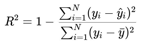
Here, y_{i} is the actual value, \hat{y}_{i} is the predicted value, and \bar{y} is the mean of all actual target values. The numerator is the model's sum of squared errors, and the denominator is the total variance of the data.
R-squared is popular because it gives an intuitive sense of how well the model fits relative to a simple average-based predictor. However, it can be misleading in scenarios with few data points or if you force the model through the origin. It can also artificially inflate when you add more features, which leads to the Adjusted R-squared metric.
Adjusted R-squared
This modifies R-squared to account for the number of features relative to the number of samples in your dataset. It attempts to penalize models that include redundant features that do not actually improve the fit.
Adjusted R-squared is particularly helpful when dealing with multiple explanatory variables, as it helps mitigate overfitting by not automatically rewarding additional parameters.
When to Choose Each Metric
MSE or RMSE: If you want a continuous measure that strongly penalizes large errors (like in many optimization frameworks) or if your application requires differentiable loss functions for gradient descent. RMSE is particularly interpretable in the original unit scale of the target variable.
MAE: When outliers are not the main focus or when a linear penalty is more suitable for your problem. MAE is robust if your data exhibits skewed distributions or strong outliers that you do not want to penalize too heavily.
MAPE: If relative errors matter more than absolute errors, for example, when predicting quantities that vary widely in magnitude or when percentage-based error interpretation is the standard for the domain.
R-squared / Adjusted R-squared: To measure how much variance is explained by your model in a more interpretable fashion. Adjusted R-squared is particularly important to consider whenever you have many features and want to guard against overfitting.
Code Example in Python
Below is a concise example illustrating how you might compute several of these metrics using scikit-learn:
import numpy as np
from sklearn.metrics import mean_squared_error, mean_absolute_error, r2_score

# Suppose y_true and y_pred are numpy arrays representing
# the actual and predicted values respectively
y_true = np.array([3.0, -0.5, 2.0, 7.0])
y_pred = np.array([2.5, 0.0, 2.1, 8.0])

mse = mean_squared_error(y_true, y_pred)
rmse = np.sqrt(mse)
mae = mean_absolute_error(y_true, y_pred)
r2 = r2_score(y_true, y_pred)

print("MSE:", mse)
print("RMSE:", rmse)
print("MAE:", mae)
print("R2 Score:", r2)
This snippet demonstrates a straightforward way to calculate some of the discussed metrics. You could also compute MAPE (as scikit-learn does not provide it directly) by doing something like:
mape = np.mean(np.abs((y_true - y_pred) / y_true)) * 100
print("MAPE:", mape, "%")
Potential Follow-up Questions
Why might you prefer RMSE over MSE?
Some engineers and data scientists prefer RMSE because it returns errors in the same unit as the original target variable. Squared errors, while beneficial for emphasizing large errors, can be less intuitive for reporting. RMSE is more interpretable in the real-world context: a model with RMSE = 2.0 means that, on average, your predictions deviate from actual values by about 2 units on the target scale.
What are the downsides of using MAPE?
MAPE can become very large or undefined when any actual values are close to zero. This is problematic for datasets containing zeros or extremely small positive targets. Additionally, it may overly penalize positive or negative errors depending on data distribution. For example, if your model overestimates very small values, MAPE can produce massive percentage errors that may overshadow the performance on the rest of the data.
When would you use Adjusted R-squared versus R-squared?
In multiple regression settings with many potential predictors, you might see that adding more features always increases R-squared, even if those features offer negligible improvements. Adjusted R-squared corrects for this by applying a penalty based on the number of predictors. If you have a large feature set relative to the number of observations, Adjusted R-squared helps you judge whether the additional variables truly improve the model’s explanatory power or if you risk overfitting.
How do you handle outliers when using these metrics?
Outliers can drastically influence MSE or RMSE because of the squared term, potentially skewing the optimization process or evaluation. MAE is more robust to outliers, but might underrepresent how problematic very large errors can be. Deciding how to handle outliers depends on the nature of your data. In some cases, you may remove them if they are truly erroneous. In others, you might employ robust methods (for instance, using MAE or using a Huber loss for training, which transitions between MAE-like and MSE-like behavior based on the magnitude of the residual).
Could you use multiple metrics for the same problem?
Yes. Often, practitioners will monitor multiple metrics, such as MSE or RMSE alongside MAE, to get both the absolute and squared error perspectives. Additionally, R-squared or Adjusted R-squared may be reported to convey how much variance is captured by the model. This multi-metric approach helps present a more nuanced understanding of model performance.