
ML Interview Q Series: What are the assumptions before applying the OLS estimator?

📚 Browse the full ML Interview series here.
Comprehensive Explanation
Ordinary Least Squares (OLS) is a widely used method for linear regression. The parameter estimates in OLS are derived by minimizing the sum of squared residuals between the observed values and the model’s predictions. A commonly cited closed-form solution for the OLS estimator of the parameter vector is
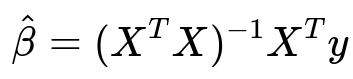
Here, X is the design matrix (with each row representing an observation and each column representing a feature), y is the vector of observed outputs, and hat(beta) is the estimated coefficients vector. The matrix X^T X must be invertible for this closed-form to exist in practice. The fundamental assumptions under which this formula provides the Best Linear Unbiased Estimates (BLUE) can be expressed and interpreted as follows.
Linearity of the Model
The model assumes a linear relationship in parameters between the features and the target variable. This means the expected value of the target (y) is a linear combination of the parameters times their corresponding features. The functional form should be correct: y = beta_0 + beta_1 x_1 + ... + beta_n x_n + error. If the true data generation process is not well approximated by a linear structure, then OLS estimates may be biased or have high variance.
Zero Mean of Errors
The error term should have an expected value of zero. Mathematically, E(error | X) = 0. This means that conditional on the explanatory variables, the errors do not systematically under or overestimate the true y values. When this assumption holds, there is no systematic bias in our estimates.
No Perfect Multicollinearity
Multicollinearity refers to the situation where some features in X are almost linear combinations of others. Perfect multicollinearity implies that at least one feature can be expressed exactly as a linear combination of other features. This makes (X^T X) non-invertible. Even near-multicollinearity can cause instability in the coefficient estimates, leading to inflated variances and making interpretation more difficult.
Homoscedasticity
The variance of the errors should be constant across all observations. Formally, Var(error | X) = constant. When the variance of the errors differs for different values of the features (heteroscedasticity), the OLS estimates remain unbiased but are no longer the most efficient (they do not have the smallest variance). In such a case, alternative methods, like Weighted Least Squares or using robust standard errors, can address heteroscedasticity.
Uncorrelated Errors
The error terms for different observations should be uncorrelated with each other. This is particularly important in time-series or spatial data, where correlation can arise over time or space. If errors are serially correlated, the straightforward calculation of standard errors is no longer valid, and specialized techniques are required to correct for this.
Normal Distribution of Errors (for inference)
For the purposes of hypothesis testing and constructing confidence intervals, it is typically assumed that the errors are normally distributed around zero with constant variance. This assumption is not strictly necessary to obtain unbiased estimates of the parameters, but it is key when deriving confidence intervals and p-values in classical linear regression inference.
Exogeneity of Regressors
The features (regressors) should be exogenous, meaning they are not correlated with the error term. If the features are correlated with the error term, it implies endogeneity, which biases the OLS estimates. In practice, endogeneity can arise from omitted variables, measurement error, or reverse causality.
How do we check if the assumptions are satisfied?
One way is to examine residual plots. For homoscedasticity, you can visualize residuals versus predicted values and check if the spread remains roughly constant. For normality of errors, statistical tests (for instance, the Shapiro-Wilk test) or Q-Q plots can be used. For correlation of errors in time-series data, methods like the Durbin-Watson test help detect autocorrelation. For multicollinearity, metrics such as the Variance Inflation Factor can shed light on how correlated the features are. If any assumption is violated, appropriate remedies—like transformations, using robust standard errors, or advanced techniques—might be needed.
Why is the normality assumption often mentioned if OLS just requires exogeneity for unbiasedness?
OLS estimates remain unbiased even if the errors are not normally distributed. However, normality is crucial when we want reliable intervals and tests based on classical linear regression theory. The derivation of t-tests, F-tests, and confidence intervals typically assumes normal residuals (along with other assumptions). If errors deviate from normality, large sample results (from the Central Limit Theorem) can still yield approximate valid inference, but for small or moderate sample sizes, significant deviations from normality can make the usual statistical inference tools inaccurate.
What happens if multicollinearity is present?
Multicollinearity leads to instability in the coefficient estimates. When one or more features are almost perfectly correlated with others, the (X^T X) matrix becomes close to singular, so the inverse can have very large entries. This results in large variances for some estimated coefficients, making them sensitive to small changes in the data. Remedies include removing redundant features, applying dimensionality reduction techniques (e.g., Principal Component Regression), or using regularization methods like Ridge Regression or Lasso.
What if the errors are heteroscedastic?
If errors have non-constant variance, the estimated coefficients remain unbiased, but the standard OLS variance estimates (and hence the related standard errors) become unreliable. Consequently, any hypothesis tests or confidence intervals might be invalid. Employing heteroscedasticity-consistent standard errors (also known as robust standard errors) can correct this. Alternatively, Weighted Least Squares can be used if there is a known structure of heteroscedasticity.
How does correlation of errors affect OLS?
In time-series or panel data, correlation among error terms is common. Standard OLS formulas for variance assume independence of the error terms. When the errors are correlated, standard errors of the estimates can be underestimated, leading to overly optimistic conclusions about significance. Techniques like Generalized Least Squares or methods that account for autocorrelation (e.g., ARIMA errors, Newey-West standard errors) can be employed in such cases to obtain consistent variance estimates.
How do we handle endogeneity?
Endogeneity arises if an explanatory variable is correlated with the error term. OLS estimates become biased and inconsistent in such scenarios. A common remedy is to use an Instrumental Variables (IV) approach, where an instrument that is correlated with the problematic regressor but uncorrelated with the error term is introduced. Two-Stage Least Squares is a common IV-based procedure that helps address endogeneity and yield consistent estimates.
Summary of Key Takeaways
OLS relies on several assumptions to ensure the estimates are unbiased, consistent, and efficient under the Gauss-Markov Theorem. In practice, it is important to diagnose these assumptions using residual analysis and other tests. When violations occur, robust or alternative regression techniques should be considered to obtain reliable estimates and valid inference.
Below are additional follow-up questions
What if the error distribution is heavily skewed or has long tails?
Heavily skewed or heavy-tailed error distributions can undermine the normality assumption traditionally used for inference. Even though OLS coefficients remain unbiased as long as the expectation of the error term is zero and the regressors are exogenous, the usual confidence intervals and hypothesis tests assume (at least in finite-sample derivations) that errors are normally distributed. If the error distribution has large tails, a few extreme points can have a disproportionate influence on the standard error estimates. In small samples, this can lead to inaccurate p-values and confidence intervals.
One practical approach is to use robust standard errors, which relax the assumption of normally distributed (and homoscedastic) errors. Another approach is to transform the dependent variable (for instance, using a log transform if positive-valued and highly skewed). If transformations fail to mitigate long-tailed behavior, alternative modeling approaches such as quantile regression or robust regression (for example, Huber or Tukey M-estimators) might be more appropriate.
A subtle issue arises when you have zero or negative values in the dependent variable that prevent a straightforward log transform. In such cases, one might consider more flexible transformations (Box-Cox, Yeo-Johnson) or specialized models (e.g., Gamma or Poisson regression if the data structure supports it). However, each transformation changes the interpretation of the regression coefficients, so the modeler must interpret results carefully.
How do outliers or high leverage points affect OLS?
Outliers are extreme data points in the target space (y-direction), whereas high leverage points are data points in the feature space (X-direction) that can strongly influence the regression fit. OLS is known to be sensitive to both because it minimizes squared residuals, and a single outlier can shift the regression line significantly.
A critical pitfall occurs when high leverage points coincide with outliers in the target. In such a scenario, one or two data points can dominate the parameter estimates, leading to unstable or misleading models. Detecting these points often involves:
Examining residual plots and leverage statistics (such as hat-values).
Calculating influence metrics like Cook’s distance or DFBETAS.
If an outlier is deemed to be valid data and not a data-entry error, the modeler might consider robust regression methods such as RANSAC or M-estimators that reduce the influence of points with large residuals. One real-world challenge is deciding which data points to exclude (if any). Removing legitimate but extreme observations can bias the model to a narrower range of typical cases, so the decision requires domain knowledge.
How does partial confounding or omitted variables that are only weakly correlated with the included features affect OLS?
Omitted variable bias arises if there is a variable that (1) significantly influences the target and (2) is correlated with the included features. Even if that omitted variable is only weakly correlated with the included features, there can still be some degree of bias in the parameter estimates. The magnitude of the bias depends on how strong the correlation is between the omitted variable and the included variables, and how much the omitted variable itself affects the target.
A subtlety is that small but systematic correlations can accumulate if multiple potentially omitted factors are present. This situation can lead to a slow drift in estimates rather than an obvious large bias from a single omitted confounder. Detecting partial confounding usually involves domain expertise: we must hypothesize possible omitted factors and determine their relationships with existing features. In practice, collecting more data or using instrumentation (Instrumental Variables) may help mitigate the bias. Regularization alone cannot fix endogeneity issues caused by correlated omitted variables—it can only reduce variance by shrinking coefficients.
How do we handle missing data in OLS regressions?
Missing data is a frequent real-world complication that can invalidate the assumptions behind OLS if not addressed appropriately. The simplest strategy is complete-case analysis, where rows containing missing values are dropped. This approach can cause sample-size reduction and introduce bias if the data are not missing completely at random.
An alternative is imputation. Simple techniques might involve replacing missing values with the mean or median, but this can distort relationships in the data. More sophisticated methods include multiple imputation, which predicts missing values using models based on other features, and then combines regression results across multiple imputed datasets for more robust parameter estimates and valid standard errors.
Pitfalls include:
If data are missing non-randomly (for example, systematically more likely to be missing for certain populations or certain ranges of the target), none of the basic methods may fully eliminate bias.
Imputation models must be carefully specified; using naive mean-imputation without considering feature-target relationships can introduce artificial correlations or reduce the variability in the data.
When might we consider transforming the data for OLS?
Transforming the dependent variable or specific features can help correct issues like non-linearity, heteroscedasticity, or heavily skewed distributions. For example, a log transform of the target can stabilize variance if the error variance grows as the target’s magnitude increases. Polynomial or interaction terms for the features can capture non-linearities that are still “linear in the parameters.” This satisfies the linear model form but allows more flexible shapes.
A practical challenge is choosing the right transformation. Domain knowledge helps in deciding whether a log transform, square root transform, or a more general Box-Cox or Yeo-Johnson transform is appropriate. Another subtlety is that transforming the target changes how residuals are interpreted. A log transform means that residuals operate in log-space, so the back-transformed predictions need to be carefully interpreted. Overlooking this can lead to incorrect estimates of error in the original scale of y.
How does OLS handle categorical variables?
OLS can incorporate categorical variables using dummy (one-hot) encoding, turning each category into a binary indicator variable. The coefficient for each indicator reflects the shift in the response relative to a baseline category. Potential pitfalls include:
Dummy Variable Trap: If we include a separate dummy for every category and an intercept, one of the indicators becomes perfectly collinear with the others. In practice, we remove one category as a reference.
Multicollinearity: When multiple categorical variables with many levels are included, or if they correlate strongly with each other, collinearity can become severe. This can inflate standard errors of the coefficients and cause interpretational challenges.
In real-world data, especially with many categories, the dimensionality can explode, causing computational challenges and high variance in the estimates. Regularization techniques or grouping less frequent categories can alleviate some of these issues.
What do we do if the relationship is not linear in the parameters but we still want to use OLS?
If the underlying relationship involves non-linear terms of parameters themselves, classical OLS assumptions (linearity in parameters) will not hold. OLS can still handle polynomial transformations or basis expansions because these are linear in the newly defined features—even though they represent a non-linear mapping of x. However, certain functional forms, like an exponential in beta (e.g., y = exp(beta_0 + beta_1 x)), are inherently non-linear in the parameters.
In such cases, we might resort to:
Non-linear least squares, which still attempts to minimize residuals but uses more complex iterative optimization procedures.
Generalized Linear Models (GLMs), if the outcome variable follows a known distribution family and a link function is defined.
Non-parametric or semi-parametric methods (splines, kernel methods) that do not impose a strict parametric structure.
One real-world challenge is balancing model flexibility against interpretability. Higher-complexity models can overfit or become very hard to interpret unless domain knowledge confirms that a non-linear specification is appropriate.