ML Interview Q Series: What are the main distinctions between Principal Component Analysis (PCA) and t-SNE for dimensionality reduction?

📚 Browse the full ML Interview series here.

Comprehensive Explanation

PCA is a linear dimensionality reduction method that looks for directions of maximum variance in high-dimensional data and projects the data onto these directions, referred to as principal components. By contrast, t-SNE is a non-linear technique that aims to preserve the local structure of data points when projecting them into a lower-dimensional representation, typically 2D or 3D for visualization purposes.

PCA uses an eigen-decomposition or singular value decomposition (SVD) approach on the covariance matrix to find orthogonal directions that capture the largest variance. These directions are the principal components, and each component explains a descending amount of variance. Once we identify these components, the original data can be projected onto them, reducing dimensionality while attempting to retain as much variance as possible.

One of the core steps in PCA is computing the covariance matrix. When you have N data samples x_1, x_2, ..., x_N in D-dimensional space, you compute their mean vector x̄ and then calculate:

where:

• x_i is the ith data sample in D-dimensional space (in plain text: x_i is dimension D),

• x̄ is the mean vector of the dataset,

• N is the total number of samples,

• \Sigma is the covariance matrix, which is D x D in size.

Then, we typically perform SVD on \Sigma to get its eigenvalues and eigenvectors. The eigenvectors corresponding to the top k eigenvalues (k < D) form the principal components onto which we project our data.

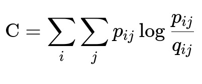
t-SNE, on the other hand, is primarily used for visualization of high-dimensional data into 2D or 3D by emphasizing local neighborhoods. It defines probabilities p_ij that measure how likely it is that point x_i would pick x_j as a neighbor if neighbors were chosen according to a Gaussian distribution centered at x_i in the high-dimensional space. Then it similarly defines q_ij in the low-dimensional map. t-SNE tries to minimize the mismatch between p_ij and q_ij using Kullback–Leibler divergence as a cost function:

where:

• p_ij is the conditional probability that x_j is near x_i in the high-dimensional space,

• q_ij is the corresponding conditional probability in the low-dimensional embedding,

• Summation over i and j means summing all pairwise relationships in the dataset.

This objective tries to make points that are close in the original high-dimensional space remain close in the low-dimensional representation, and those that are far apart in the high-dimensional space remain less likely to end up close in the lower-dimensional embedding.

Because of these differences, PCA is faster, deterministic, and focuses on capturing global variance in a linear subspace. t-SNE is slower, non-deterministic (due to random initialization and stochastic gradient-based optimization), and provides visually interpretable clusters by preserving local neighborhoods but does not guarantee global structure preservation.

Practical Implementation Aspects

PCA can be easily applied to large datasets without too high a computational cost. It is also straightforward to interpret the principal components, which can help you understand the underlying linear patterns in your data. Furthermore, PCA is deterministic, so the same data always produces the same principal components.

t-SNE is usually considered for visualization tasks where you want to discern local clustering and neighborhood relationships in high-dimensional data. However, it is more computationally expensive and can have multiple hyperparameters, such as perplexity, that significantly affect the resulting visualization. Moreover, slight changes in random seed or hyperparameters can lead to different final embeddings, which can confuse interpretation.

t-SNE is generally not used for tasks requiring a linear transformation back to the original feature space or for large-scale feature engineering. PCA, on the other hand, is often used to reduce dimensionality prior to modeling, or for exploratory data analysis as a linear technique that allows partial reconstruction of the original data.

Potential Follow-Up Questions

How do the hyperparameters of t-SNE impact its results?

t-SNE’s main hyperparameters include perplexity, early exaggeration factor, and learning rate. Perplexity controls the effective number of neighbors considered when computing the conditional probabilities in the high-dimensional space. A low perplexity might lead to very tight clusters, while a very high perplexity can cause more global mixing, potentially losing local detail. Early exaggeration helps the model form distinct clusters in early optimization steps. The learning rate must be tuned carefully—too high can cause the model to diverge, and too low can slow down the convergence.

Because t-SNE’s optimization is stochastic, the final embedding can differ across runs when you vary the random seed or hyperparameters, so it is common to try multiple runs and compare results.

Under what circumstances might PCA be preferred over t-SNE?

PCA is often preferred when interpretability of components and computational efficiency are important. For instance, if you are working on a large dataset and want to quickly reduce dimensionality to feed into another algorithm, PCA can be a sensible choice. PCA also gives you direct principal components that can be interpreted in the original feature space (e.g., which features contribute the most to each component). Moreover, if you need to invert the transformation or reconstruct approximate original data from the reduced dimension, PCA allows this since it is linear.

In contrast, t-SNE is primarily used for visualizing the data in lower dimensions (often 2D). If your goal is strictly visualization and you want to preserve local structure, t-SNE might produce more insightful clusters. However, it will not yield an easy linear mapping back to the original space.

Why do t-SNE embeddings sometimes appear clustered, even if no real clusters exist?

t-SNE emphasizes local structure and can create visually distinct clusters because it tries to push dissimilar points far apart. When perplexity or other hyperparameters are not well calibrated, or the intrinsic dimensionality is too high, t-SNE might artificially enforce clusters. It is important to cross-check such clustering visually with known labels, or compare across multiple runs and parameter sets.

Is t-SNE scalable to very large datasets?

Pure t-SNE implementations have a computational cost that can become prohibitive for very large datasets, because they rely on pairwise computations (often O(N^2)). There are approximate implementations and optimizations (such as Barnes-Hut t-SNE and other variations) that improve performance, but scaling to tens of millions of data points can still be challenging. In contrast, PCA can handle very large datasets more readily, especially if you use incremental PCA or randomized SVD methods.

Does PCA capture non-linear relationships the same way t-SNE does?

PCA only captures linear relationships in data, as it relies on covariance structure. Non-linear structures, like manifolds or more complex data distributions, may not be well-represented by a linear projection. t-SNE explicitly focuses on preserving local neighborhoods and can capture more complex structures, such as curved manifolds. Therefore, for data with strong non-linear manifold structures, t-SNE may reveal patterns that PCA cannot.

Can we use PCA before t-SNE?

It can be advantageous to first use PCA to reduce the dimensionality from a very high dimension (e.g., thousands of features) down to a manageable size (like 30-50 principal components), and then run t-SNE on that lower-dimensional representation. This approach saves computational resources and can sometimes help t-SNE converge faster and more reliably, although in some cases it might remove interesting structure that t-SNE could otherwise discover.

Example Code Snippet for PCA and t-SNE in Python

import numpy as np
from sklearn.decomposition import PCA
from sklearn.manifold import TSNE

# Sample data (N=100 samples, D=50 features)
X = np.random.rand(100, 50)

# PCA to 10 components
pca = PCA(n_components=10)
X_pca = pca.fit_transform(X)

# t-SNE to 2 components (for visualization)
tsne = TSNE(n_components=2, perplexity=30, random_state=42)
X_tsne = tsne.fit_transform(X_pca)  # Often do PCA first then t-SNE

print("PCA shape:", X_pca.shape)   # (100, 10)
print("t-SNE shape:", X_tsne.shape)  # (100, 2)

In practice, you might adjust the perplexity, run multiple initializations, or skip the PCA step if you suspect it might remove important structure.