
ML Interview Q Series: What are the differences between minimizing squared error vs. absolute error, and when is each suitable?

📚 Browse the full ML Interview series here.
Short Compact solution
Both metrics measure how far predictions are from targets, but squared error (MSE) squares each discrepancy before averaging, whereas absolute error (MAE) uses the absolute value of the differences. Because MSE squares errors, large deviations become much more significant, so MSE is suitable if avoiding large errors is particularly important. Outliers have a bigger impact on MSE than on MAE, making MAE more robust. From a computational point of view, MSE is simpler to handle for gradient-based optimization, since its derivative is linear in the residual, whereas MAE has a sign function component that complicates gradient calculations. MSE is also tied to the assumption of normally distributed errors and is minimized by the conditional mean, while MAE is minimized by the conditional median. Consequently, models that must handle outliers effectively often benefit from MAE, whereas problems where large deviations are especially costly, or where a Gaussian error assumption is appropriate, favor MSE.
Comprehensive Explanation
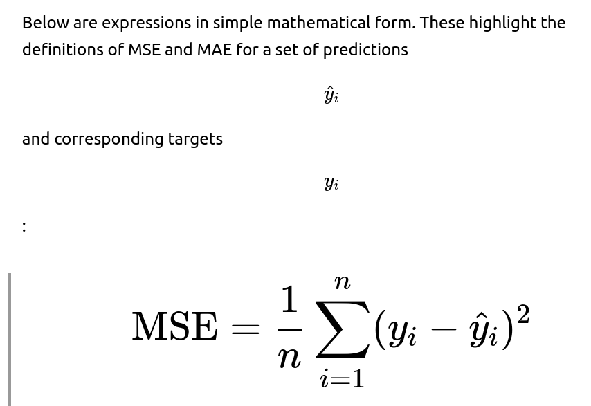
Squared error is typically referred to as Mean Squared Error (MSE). It is computed by taking the difference between the predicted values and the actual values, squaring these differences, then averaging. Because of the squaring step, large discrepancies grow rapidly, which means the model is heavily penalized for predictions that stray far from their true targets. This approach makes sense when punishing big mistakes much more than smaller ones, and it aligns with Gaussian error assumptions often used in statistical modeling.
Absolute error is generally called Mean Absolute Error (MAE). It is calculated by taking the absolute value of the difference between the predicted values and the actual values and then averaging these absolute residuals. Since the absolute value grows more linearly, there is less penalty for extremely large deviations relative to MSE. Models optimizing MAE effectively reduce overall deviations without disproportionately emphasizing individual large errors. Consequently, MAE is more robust to outliers, as one or two extreme values do not dominate the loss nearly as much as with MSE.
From an optimization perspective, MSE offers a straightforward gradient computation. The derivative of a squared difference with respect to the model parameters is continuous and does not involve sign operations. In contrast, the absolute value function is non-differentiable at zero, which makes the gradient-based optimization a bit trickier for MAE. Modern solvers and frameworks can handle MAE as well, but there is a historical preference for MSE due to simpler calculus and well-studied convergence properties under Gaussian assumptions.
Another important distinction is that MSE is minimized by the conditional mean of the target distribution. In other words, if you want to predict the value that best minimizes MSE, you would use the mean of the distribution of possible outcomes. On the other hand, MAE is minimized by the conditional median. This property directly influences the model’s interpretability and use cases. If you care more about capturing the “middle” of a distribution (especially with skewed data or outliers), predicting the median might be preferred, aligning with MAE. If the data is assumed to have more symmetrical distributions, or you want to account for the largest errors heavily, MSE provides an appropriate framework.
In terms of real-world usage, MSE can be the right choice if:
You assume or empirically observe that errors follow (approximately) a normal distribution.
You can afford to penalize large deviations disproportionately.
Computation of gradients needs to remain straightforward.
MAE might be a better choice when:
The data has non-trivial outliers or a heavy-tailed distribution.
You want a more median-like estimator.
You value robustness to a handful of extreme target values.

Even though both losses can be used in practice, nuances in data distribution, model behavior around outliers, and ease of optimization often guide the choice of one over the other.
Follow-up question: Why is MSE often easier to handle in gradient-based optimization?
When you compute the derivative of the squared loss function, the gradient is simply proportional to the difference between the prediction and the target, which remains a smooth function across the entire real line. In contrast, the derivative of the absolute loss involves the sign of the residual, which changes abruptly at zero and is not defined at that point. While this does not make MAE impossible to optimize, it can introduce subtleties in gradient-based methods, especially if you rely on purely analytical updates. Libraries such as PyTorch or TensorFlow handle subgradients (or approximate derivatives) for the absolute value function, so modern optimizers can still handle MAE with minimal issues. Historically, however, MSE’s smooth nature was more convenient and became standard in many algorithms.
Follow-up question: How do assumptions about data distributions influence the choice between MSE and MAE?
Squared error aligns with the assumption that residuals (differences between predictions and actual values) are normally distributed. Minimizing MSE in this setting is equivalent to maximizing the likelihood of the observed data under a Gaussian noise model. On the other hand, absolute error aligns with a Laplacian (or double exponential) error model. If you have reason to believe your data has fatter tails or you observe that a few outliers are drastically skewing predictions under MSE, switching to MAE could produce more stable results. Essentially, MSE will be the best unbiased estimator for the mean if the noise is Gaussian, while MAE will act as the best unbiased estimator for the median under a Laplacian model.
Follow-up question: Could we combine both approaches in a single loss function?
Yes, one common approach is the Huber loss (sometimes called the "smooth L1" loss), which behaves like MSE for small residuals and like MAE for large residuals. This gives a balance: small errors are penalized quadratically, ensuring smooth gradients, but large errors are penalized linearly, giving some robustness to outliers. Conceptually, Huber loss transitions from one regime to another based on a threshold parameter, which can be tuned to the scale of the dataset’s noise.
Follow-up question: What are some practical tips for implementing MSE and MAE in a deep learning framework?
In PyTorch, for example, you can use built-in loss functions:
import torch
import torch.nn as nn

# Suppose preds and targets are tensors of shape [batch_size, ...]

mse_loss_func = nn.MSELoss()
mae_loss_func = nn.L1Loss()  # L1Loss is another name for MAE

mse_value = mse_loss_func(preds, targets)
mae_value = mae_loss_func(preds, targets)
Internally, these are computed as described mathematically. For MSE, PyTorch uses a smooth gradient that remains continuous. For MAE (referred to as L1Loss in PyTorch), the framework implements subgradient methods for absolute values. Similar APIs exist in TensorFlow, Keras, and other libraries.
When training, you might select MSE or MAE depending on your data distribution and the model’s need to either strongly penalize large errors (MSE) or resist outlier distortions (MAE). Make sure to experiment with both, especially if you suspect non-Gaussian noise in your data, or if you observe that outliers degrade performance.


Below are additional follow-up questions
How do MSE and MAE extend to multi-dimensional or multi-output regression tasks?
When you have multiple targets to predict simultaneously (for example, predicting both height and weight in a single model), you typically compute the loss for each target dimension and then average across dimensions.
Using MSE: You would sum (or average) the squared errors for each target dimension. For instance, if you have two targets per sample, you compute the squared difference for each, add them, and then average over all samples. This effectively treats each dimension equally unless you introduce separate weights.
Using MAE: Similarly, you can compute the absolute differences for each target dimension, sum (or average) them, and then average across all data points.
Because multi-output tasks can involve targets with different scales, it may be prudent to normalize or weight each dimension’s contribution to the final loss. Otherwise, the dimension with larger numeric range might dominate the combined loss.
Pitfalls or Edge Cases
If one dimension is in the tens (e.g., price in dollars) and another is in the thousands (e.g., number of transactions), the larger-scale dimension can overshadow the smaller-scale dimension if you do not normalize or re-weight them.
If you equally weigh each dimension without carefully examining the distribution, important but lower-scale targets might be underemphasized.
When you have correlated outputs, a single aggregated MSE or MAE might ignore potential covariance effects unless carefully accounted for, though that often requires more advanced methods than standard regression loss functions.
In what scenarios could using MSE or MAE in a classification problem be applicable, and what are the caveats?
Typically, MSE or MAE are not the most common choices for classification tasks—classification usually relies on cross-entropy or logistic loss. However, there might be scenarios where the outputs of your model are unbounded continuous values that you subsequently threshold or interpret as probabilities.
Using MSE or MAE with label encoding: If you encode classes as numeric values (e.g., 0 or 1 for binary classification), you can measure the difference between the continuous output and the encoded label. However, such an approach can lead to slower or less stable convergence since the signal for improvement may be weaker compared to cross-entropy’s log-based gradient.
Using MSE or MAE for ordinal classification: If you have an ordinal classification task (where classes have a natural ordering, like small < medium < large), sometimes MAE or MSE can be employed if you encode each class with a numeric rank. This can make sense when misclassifying an adjacent category should be penalized less than misclassifying a distant category.
Pitfalls or Edge Cases
Using MSE or MAE directly on 0/1 labels often gives slower convergence compared to logistic loss, and it may not capture the probabilistic interpretation well.
If the data is highly imbalanced, raw MSE or MAE might not reflect meaningful performance.
Interpreting the continuous output as a probability requires careful calibration. If you just interpret any output above 0.5 as class 1, MSE or MAE may not align with a well-calibrated probability distribution.
How can we scale or normalize MSE and MAE for different datasets or tasks, and why might that be beneficial?
Scaling or normalizing these metrics can help compare performance across tasks or features with different numeric ranges. Common approaches:
Division by data variance: Sometimes you normalize by the variance of the target variable. This helps interpret whether the model is performing better than a naïve “predict the mean of the target” strategy.
Relative/Percentage Errors: You might use something like Mean Absolute Percentage Error (MAPE) or Root Mean Squared Percentage Error (RMSPE). This puts errors in the context of the magnitude of the target, helpful in finance or demand forecasting where relative differences matter more.
Pitfalls or Edge Cases
If your data includes zeros or near-zeros, MAPE or percentage-based metrics can blow up or become undefined.
Normalizing by variance is unhelpful if the target distribution is heavily skewed or if the variance is extremely small/large.
Over-normalization can hide absolute scale errors that matter in real-world applications.
When might log-based errors or other transformations be more appropriate than MSE or MAE?
In certain domains—particularly where target values can span several orders of magnitude, such as in financial prices or population sizes—logarithmic errors (e.g., MSE of the log of predictions vs. the log of actuals) can be more relevant.

. This penalizes relative errors instead of absolute differences in the original scale.
Benefit: Predicting in log-space often reduces the influence of large target values and focuses on ratio-based accuracy.
Pitfalls or Edge Cases
You cannot apply a log transform when target values are zero or negative. You would need to shift the targets or handle them separately.
A predicted negative value is invalid in log-space, so the model must remain constrained or carefully parameterized.
The transformation can complicate interpretability if stakeholders expect predictions in the original linear scale.
Could MSE or MAE lead to suboptimal solutions if the underlying assumptions about the data do not hold?
Yes, both MSE and MAE assume certain distributions or behaviors:
MSE relies heavily on the assumption of a Gaussian error structure, so if the actual error distribution is highly skewed or heavy-tailed, MSE might over-penalize outliers. This can lead to a model that tries too hard to fix the outliers rather than focusing on the bulk of the data.
MAE implicitly assumes a Laplacian error distribution. If the real-world distribution is quite different, MAE might not align with the best metric for your application.
Pitfalls or Edge Cases
Real data often has mixed distributions or multi-modal outcomes, making both MSE and MAE imperfect.
If your data has complex outliers (e.g., systematic but infrequent phenomena), neither MSE nor MAE alone may capture the situation well. A specialized loss or outlier detection pre-processing might be more appropriate.
Overemphasizing the chosen loss function can bias the model away from objectives that are important in practice, such as consistent performance across subgroups.
What special considerations arise for real-time inference or streaming data when using MSE or MAE?
When you have streaming data or real-time predictions, the distribution of inputs and targets may shift over time (concept drift).
Model Adaptation: If the underlying distribution changes, the historical MSE or MAE might become stale, and the model may need continual or online training. Monitoring MSE or MAE over time helps detect data drift.
Rolling window: Some systems compute a rolling MSE or MAE over a fixed window of recent predictions to adapt quickly if the underlying patterns shift.
Computational Efficiency: In real-time settings, you must ensure your computation of the loss does not become a bottleneck. Typically, MSE and MAE are still cheap to compute, but handling large volumes of streaming data might require incremental updates.
Pitfalls or Edge Cases
Using a static model in a rapidly changing environment can lead to steadily growing MSE or MAE. You need mechanisms to detect and handle drifting concepts or anomalies.
If outliers appear sporadically in streaming data, MSE might spike heavily and overshadow the average, whereas MAE might be slower to reflect moderate but persistent changes in the mean trend.
When might we want a custom loss function that weighs different errors instead of standard MSE or MAE?
Some real-world problems assign different costs to underestimation vs. overestimation, or penalize errors more severely in certain ranges. In such cases, a standard symmetrical loss might not accurately capture the business or domain requirements.
Example: Over-forecasting production might be less costly than under-forecasting because running out of inventory is very expensive. A custom asymmetric loss can reflect that difference.
Another Example: In medical applications, a false-negative could be riskier than a false-positive for a specific health condition, prompting a specialized penalty structure.
Pitfalls or Edge Cases
Designing custom loss functions without rigorous validation can lead to odd optimization behavior or unintended local minima.
You must carefully engineer and tune weight coefficients; an extreme weighting scheme might hamper the model’s overall learning of typical patterns.
Some specialized losses can be more complex to differentiate, requiring approximate or numerical methods that might slow training.
How should we handle scenarios where multiple target variables have drastically different scales but are jointly predicted with a single MSE or MAE?
In multi-task or multi-output regression, if one target is naturally around 1,000 while another is around 0.1, a raw MSE or MAE might be dominated by the large-scale target.
Normalization by each target’s standard deviation: One common practice is to normalize or standardize each dimension so that each target has roughly the same scale. Then the combined MSE or MAE is more equitable.
Weighting: Assign a weight to each target dimension based on domain importance or typical scale. You might say that the first dimension’s error counts for 30% and the second dimension’s for 70%, etc.
Pitfalls or Edge Cases
If you standardize each target variable, be sure to transform predictions back to original scales before final deployment.
Overweighting or underweighting certain targets can degrade performance on other tasks if you haven’t validated the weighting strategy.
If the targets are correlated, normalizing each dimension individually might ignore cross-correlations. A more advanced approach might simultaneously account for covariance.
If the data includes mixed discrete and continuous targets, can MSE or MAE handle that? What approaches might be better?
Sometimes you have a hybrid output where part of it is continuous (like a regression variable) and part is categorical (like a class label or an integer count).
Using MSE/MAE on continuous part only: For the discrete part, you generally would rely on classification losses (e.g., cross-entropy). The overall loss may be the sum of the classification loss for the discrete target and the MSE/MAE for the continuous target.
Better Approach: A multi-objective loss can unify these. You could combine a cross-entropy term for the classification piece and an MSE or MAE term for the continuous regression piece.
Pitfalls or Edge Cases
Simply concatenating discrete and continuous targets and applying an MSE or MAE directly (by encoding discrete classes as numbers) typically leads to suboptimal training, as the discrete dimension does not behave like a continuous variable.
Weighting each portion of the loss is critical to ensure the model trains effectively for both tasks. If you overly emphasize one component, performance on the other might degrade significantly.