
ML Interview Q Series: What does t-Distributed Stochastic Neighbor Embedding do, and how does it work in reducing dimensionality?


📚 Browse the full ML Interview series here.
Comprehensive Explanation
t-Distributed Stochastic Neighbor Embedding (t-SNE) is a method designed for visualizing high-dimensional data by mapping it into a lower-dimensional space (often 2D or 3D) in a way that tries to preserve local structures or neighborhoods. The result is commonly used for exploratory analysis, where we want to see clusters or manifolds in a visibly interpretable way.
t-SNE begins by converting distances between high-dimensional points into conditional probabilities. In the original high-dimensional space, each pair of points x_i and x_j has an associated similarity measure p_j|i. This is done by using a Gaussian distribution that is centered on each point x_i. The similarity distribution in high-dimensional space is then matched to a corresponding distribution in the low-dimensional space, except the low-dimensional distribution uses a heavy-tailed Student’s t distribution to handle crowding effects better.
Below is the high-dimensional distribution for each pair, expressed in a core formula that is central to the understanding of t-SNE:
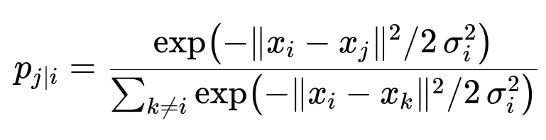
The parameter x_i is the position of point i in high-dimensional space, x_j is the position of point j, and sigma_i is the variance of the Gaussian centered on x_i. The perplexity, which is a user-defined parameter, influences sigma_i so that each local neighborhood matches the user’s desired effective number of neighbors.
t-SNE then defines a low-dimensional distribution for each pair of points y_i and y_j in the embedding space (2D or 3D). It uses a heavy-tailed distribution (specifically, the Student’s t distribution) to combat the crowding problem. The method tries to minimize the difference between these two distributions using the Kullback-Leibler (KL) divergence. This cost function, which is also central to the concept of t-SNE, is typically:

Here p_{ij} is the joint probability in the high-dimensional space (symmetrized from p_j|i and p_i|j), and q_{ij} is the corresponding joint probability in the low-dimensional space (using the Student’s t distribution). The algorithm iteratively updates the low-dimensional coordinates y_i and y_j to minimize this cost. Through gradient descent, similar points end up close to one another in the 2D or 3D embedding, and dissimilar points stay farther apart.
Because t-SNE emphasizes local similarity, it excels at revealing clusters or manifolds in high-dimensional data. However, it is not meant for strictly preserving global distances. It instead focuses on preserving local neighborhoods.
How does perplexity influence the distribution computations in t-SNE?
Perplexity is an important hyperparameter that guides the choice of sigma_i in the Gaussian distribution of the high-dimensional space. A higher perplexity setting increases sigma_i, so each point’s neighborhood grows larger. In practice, setting perplexity too low can cause the algorithm to produce very tight clusters and may fail to capture broader structures. Setting perplexity too high can lead to overlapping clusters and loss of local detail. Empirical recommendations often place perplexity in a range of 5 to 50, but this will always depend on the specific data.
Why does t-SNE use a Student’s t distribution instead of a Gaussian in the low-dimensional space?
The Student’s t distribution with one degree of freedom is a heavy-tailed distribution. This design choice combats the “crowding problem,” where points in low-dimensional space can end up too close together, making distances there unrepresentative of the actual high-dimensional local similarities. By using heavier tails, the distribution in the low-dimensional space allows moderate distances in the embedding to still be represented without requiring large separation of clusters. This helps maintain small local neighborhoods while still preserving separation between distinctly different clusters.
What are some potential pitfalls of t-SNE?
One pitfall is that t-SNE can produce visually appealing clusterings, but those clusters might be easily misinterpreted as clearly separated groups. The local neighborhoods are well preserved, but global distances are not always to be trusted. Another pitfall is parameter sensitivity: changing perplexity or the number of iterations can yield drastically different embeddings. Finally, t-SNE can be computationally expensive for large datasets, requiring specialized approximations (like Barnes-Hut t-SNE or other variants) to make it scale more efficiently.
How do you interpret a t-SNE plot?
t-SNE is best interpreted in terms of local proximity. Points or regions that appear close together in the final embedding are likely to be similar in the original high-dimensional feature space. However, global distances and the relative positioning of separate clusters in the 2D or 3D plot are not necessarily meaningful. One cannot assume that the distance between two well-separated clusters is a faithful measure of how different they are in the original space.
When can t-SNE produce misleading results?
t-SNE can be misleading if the perplexity is poorly chosen or if the algorithm’s random initialization leads to a suboptimal embedding. If the data inherently lacks local manifold structure or is extremely noisy, t-SNE may produce spurious clusters. Additionally, small sample sizes or inappropriate parameter settings (too many iterations or too few) can reveal patterns that are mere artifacts.
How can t-SNE be accelerated?
Standard t-SNE has a computational complexity that is roughly O(N^2) in naive implementations, where N is the number of data points. This can be prohibitive for large datasets. Approximation techniques such as Barnes-Hut t-SNE or FIt-SNE reduce complexity by approximating pairwise interactions. Barnes-Hut t-SNE uses a quadtree (in 2D) or octree (in 3D) for approximating forces, effectively reducing the complexity to about O(N log N). Other approaches, such as using GPUs or distributing calculations, can further speed up the process.
Example Implementation in Python
Below is a simple demonstration of using t-SNE in Python with scikit-learn. This is a minimal code example:
import numpy as np
from sklearn.manifold import TSNE

# Example high-dimensional data
X = np.random.randn(100, 50)  # 100 samples, 50 features

# Create a TSNE instance with certain hyperparameters
tsne = TSNE(n_components=2, perplexity=30, learning_rate=200, n_iter=1000, random_state=42)

# Fit and transform
X_embedded = tsne.fit_transform(X)

print("Shape of the low-dimensional embedding:", X_embedded.shape)
The above code generates a random matrix X with 100 samples and 50 features. It then applies t-SNE to map these points into 2 dimensions with a perplexity of 30 and a learning_rate of 200. The result X_embedded is a 2D array for visualization or further analysis.
By tuning perplexity, learning_rate, and n_iter, one can adjust how the final embedding appears. But always keep in mind the interpretative limitations: local clusters are significant, while large-scale distances are generally unreliable.