
ML Interview Q Series: What does the concept of Ensemble Nyström methods refer to, and how do they differ from the standard Nyström approach for approximating kernel matrices?


📚 Browse the full ML Interview series here.
Comprehensive Explanation
Ensemble Nyström algorithms extend the standard Nyström method for approximating large kernel matrices in situations where kernel computations become prohibitively expensive as the dataset size increases. The core idea behind the Nyström approach is to sample a smaller subset of the data points (often referred to as landmark points), construct an approximation of the full kernel matrix from that subset, and use this low-rank representation in downstream tasks such as classification or regression. Ensemble Nyström methods further improve upon this by combining multiple separate Nyström approximations, each derived from different subsets of the data, to achieve a more robust and accurate approximation.
The key to understanding Ensemble Nyström methods is to see how different subsets of data can capture different aspects of the kernel space. By averaging or otherwise combining multiple approximations, the overall result tends to be better than relying on a single subset. This is somewhat analogous to ensemble methods in machine learning, where multiple estimators reduce variance and improve overall generalization.
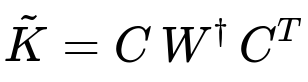
A concise expression of the standard Nyström approximation for a kernel matrix K can be written in its low-rank form. If we take a subset of m columns (and corresponding rows, since K is symmetric and positive semi-definite) of K, we can form a submatrix C of size n by m and a smaller submatrix W of size m by m. The approximate kernel matrix can be expressed as:
where:
C is the sub-block of K formed by taking all rows but only the columns corresponding to the m chosen landmark points.
W is the kernel matrix restricted to the m chosen points (an m-by-m matrix).
W^{\dagger} indicates the Moore-Penrose pseudoinverse (or another stable inverse approximation if W is invertible).
K is the original n-by-n kernel matrix.
n is the total number of samples.
m is the smaller number of landmark points (m << n).
In an ensemble version of the Nyström method, one performs this submatrix construction multiple times (potentially with different random subsets or different sampling techniques) and then combines the resulting low-rank approximations. The simplest way to combine these approximations is typically by taking the average of the approximate kernel matrices, although more sophisticated combination strategies exist (such as weighted averaging, depending on the sampling distribution).
One rationale behind combining multiple Nyström approximations is to reduce the variance that arises from randomly choosing a single subset of landmark points. If each subset alone offers a decent (but imperfect) approximation, averaging over several approximations can lead to a more accurate representation of the underlying kernel structure.
Implementing Ensemble Nyström approaches can be done by splitting your data into different subsets, computing partial kernel approximations on each subset, and then carefully merging them. Although this often increases computational requirements compared to a single-shot Nyström method, it may still be considerably cheaper than computing the full kernel matrix when n is extremely large. Furthermore, parallelization is straightforward because each subset can be processed independently, making the method highly scalable.
Below is a brief illustrative example (in Python) of how one might outline an Ensemble Nyström approximation. This is just a sketch, focusing on the conceptual steps rather than a fully optimized or production-level implementation.
import numpy as np
from numpy.linalg import pinv

def compute_nystrom_approx(K_partial, rows, columns):
    # K_partial is the submatrix of K indexed by 'rows' x 'columns'
    # K_diag is the submatrix of K indexed by 'columns' x 'columns'
    C = K_partial
    W = K_partial[np.ix_(columns, columns)]
    W_inv = pinv(W)  # or a stable inverse approximation
    return C @ W_inv @ C.T

def ensemble_nystrom(kernel_func, X, subset_sizes, num_ensembles=5):
    # kernel_func: a function that computes the kernel K(x_i, x_j)
    # X: the entire dataset of size n
    # subset_sizes: a list or single value for how large each subset of landmark points is
    # num_ensembles: number of approximations to combine

    n = len(X)
    K_ensemble_sum = np.zeros((n, n))

    for _ in range(num_ensembles):
        # Randomly pick a subset of indices
        subset_indices = np.random.choice(n, size=subset_sizes, replace=False)

        # Construct partial kernel
        # K_partial: shape is (n, m)
        K_partial = np.array([[kernel_func(X[i], X[j]) for j in subset_indices] for i in range(n)])

        # Compute approximate kernel matrix
        K_approx = compute_nystrom_approx(K_partial, range(n), range(len(subset_indices)))

        # Accumulate the approximations
        K_ensemble_sum += K_approx

    # Average the results
    return K_ensemble_sum / num_ensembles
One advantage of Ensemble Nyström algorithms is their robustness. If a single subset inadvertently omits certain crucial points, it might provide a poor approximation in regions of the input space where the kernel has complex structure. By drawing multiple subsets, the ensemble is more likely to capture the important regions of the kernel space. Another advantage is parallelism: each approximation can be computed independently on separate machines or cores.
A subtle issue to watch out for is that combining many approximations can lead to increased memory usage, since each partial approximation might be quite large. One must carefully manage both time and space complexity. Another consideration is how to choose subset sizes and sampling distributions. Some strategies select landmark points more intelligently by leveraging clustering or other data-dependent approaches to ensure a more representative subset.
When it comes to real-world applications, Ensemble Nyström methods often appear in large-scale kernel regression or kernel-based machine learning pipelines. They are particularly beneficial when dealing with vast datasets and when exact kernel computations become infeasible. The final tradeoff often balances accuracy improvements from multiple approximations against the additional computational overhead.
How They Differ from the Standard Nyström Approach
They explicitly construct multiple, independently sampled Nyström approximations and aggregate them. In contrast, the standard Nyström approach typically relies on a single set of landmark points, which can be sufficient but might be sensitive to the particular sample chosen. Ensemble methods reduce this variability and can deliver a more consistent approximation across different runs.
Potential Follow-up Questions
How does an interviewer probe deeper into these methods?
How do you choose the best subset size for each Nyström approximation?
In practice, the user might start with a rule of thumb or rely on cross-validation. The tradeoff is that choosing a larger subset improves accuracy but also requires more computation and memory. With ensemble methods, one might even adjust the subset sizes across different runs (e.g., mixing large and small subsets) to capture different resolutions of the data.
Are there any risks in averaging kernel approximations from very differently sized subsets?
If some subsets are significantly smaller than others, they might lead to approximations that are too coarse. Large subsets generally provide finer-grained approximations but cost more to compute. In practice, the user might weigh each approximation by its subset size or by an error estimate, ensuring that the ensemble is not dominated by poorly sampled approximations.
Does the choice of sampling strategy affect Ensemble Nyström performance?
Random uniform sampling is a common baseline, but more sophisticated methods may involve leverage-score sampling or other data-dependent techniques to select the most informative landmark points. These strategies often yield more accurate approximations, but they can be more expensive to implement since they require additional computations or data insights beforehand.
Can Ensemble Nyström be parallelized effectively?
Yes. Each approximation can be computed in parallel, since it involves sampling a different set of landmarks and partially evaluating the kernel. After the separate approximations are computed, one can combine the results (for example, by averaging) in a subsequent merge step. This structure suits large-scale distributed systems very well.
How does one ensure numerical stability in the inversion of W?
Numerical stability can be addressed by adding a small regularization term (e.g., lambda on the diagonal) to W before inversion. This corresponds to a regularized kernel approximation, which can help avoid issues when W is nearly singular. Alternatively, using stable matrix factorizations (like QR or SVD) instead of directly inverting W is also common.
These nuances highlight the sort of deep knowledge an interviewer would expect for a senior machine learning position at a top tech firm. Ensemble Nyström algorithms, just like other ensemble strategies, underscore the idea that combining multiple approximations can provide better overall performance than relying on a single instance of an approximate algorithm.