
ML Interview Q Series: What factors motivate the use of Probability Calibration in machine learning models?


📚 Browse the full ML Interview series here.
Comprehensive Explanation
Probability calibration is employed to ensure that the predicted probabilities output by a model correspond well to the true likelihood of outcomes. In many classification scenarios, models might be good at ranking predictions (i.e., correctly distinguishing positive vs. negative examples) but may not produce probabilities that faithfully mirror real-world frequencies. For example, a model could consistently predict a 0.9 probability for an event, but in reality, it might occur only 70% of the time. Probability calibration helps to bridge this gap, making the model’s probability estimates more reliable for downstream decision-making.
Well-calibrated probabilities are critical in applications that demand an accurate understanding of uncertainty, such as medical diagnostics (to determine risk levels), finance (to assign probabilities of default), or recommendation systems (to indicate confidence). Even when a model has high accuracy, if its confidence levels are misleading, stakeholders can misinterpret the risk or trust decisions incorrectly. This is why metrics and methods focusing on calibration are an essential part of the modern machine learning pipeline.
Common Metrics to Gauge Calibration
One widely used metric is the Brier Score, which measures the mean squared difference between predicted probabilities and the actual outcomes (0 or 1).
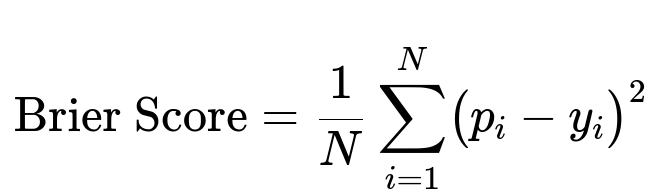
Where:
N is the number of samples.
p_i is the predicted probability of the positive class for the i-th sample.
y_i is the actual label for the i-th sample (0 or 1).
The lower the Brier Score, the better the calibration and accuracy of the model’s probabilistic predictions. Other approaches include Expected Calibration Error (ECE) and visually inspecting reliability diagrams. Reliability diagrams plot predicted probabilities on the x-axis and the actual fraction of positives on the y-axis; a perfectly calibrated model’s plot should align with the diagonal line y = x.
Approaches to Achieve Probability Calibration
Various algorithms can calibrate probabilities post-hoc without retraining the original model’s core parameters:
Platt Scaling (Logistic Calibration): Fits a logistic function on top of the model’s outputs. If a model outputs a score f(x), Platt scaling estimates parameters alpha and beta to transform that score into a probability p_cal = 1/(1 + exp(-(alpha + beta*f(x)))).
Isotonic Regression: A non-parametric method that maps the predicted scores to probabilities in a piecewise-constant, monotonically increasing fashion. This can sometimes yield better calibration than Platt scaling, especially when the relationship between model scores and actual probabilities is not strictly logistic.
Temperature Scaling (for neural networks): A special case of Platt scaling with beta = 1/T and alpha = 0, so that p_cal = softmax(z / T), where z is the network’s output logits. Adjusting T helps correct over-confident or under-confident predictions, especially in deep learning contexts.
These methods act as “layers” applied to the outputs of the underlying classification model. They do not typically change the decision boundary but rather rescale the probabilities for improved alignment with real-world frequencies.
Pros and Cons of Probability Calibration
Pros:
Helps decision-makers trust the model’s confidence scores.
Improves performance in applications requiring well-grounded probabilities (risk assessment, resource allocation, etc.).
Does not force you to retrain the original classifier from scratch; calibration layers can be fit afterward.
Cons:
Requires sufficient validation data to learn calibration parameters reliably.
Overfitting can occur if the calibration set is small.
Might slightly degrade the model’s discrimination (ranking capability) if not done carefully, though typically this effect is minimal compared to the benefit of well-calibrated probabilities.
Potential Follow-Up Questions
How do you measure the calibration quality of a model beyond the Brier Score?
You can use metrics like Expected Calibration Error (ECE) or Maximum Calibration Error (MCE). These metrics break down predictions into bins based on their predicted probability (e.g., 0.0–0.1, 0.1–0.2, etc.) and then compute how far each bin’s average predicted probability is from its empirical frequency of positives. A well-calibrated model will have small differences within each bin. Visually, reliability diagrams are also helpful to see if the calibration curve deviates significantly from the diagonal.
What are some practical scenarios where probability calibration is especially important?
Any scenario where decisions hinge on precise probability estimates benefits from calibration. Examples include:
Medical diagnostics, where a physician might administer treatments based on the likelihood of disease.
Credit risk assessment, where a bank might approve or deny loans based on default probabilities.
Weather forecasting, where accurate probability estimates of rain or storms affect planning.
Fraud detection, where the threshold for investigating fraudulent activity depends on the predicted probability of fraud.
In these cases, an uncalibrated but high-accuracy model could be risky, because stakeholders would rely on probability outputs that may not reflect the actual likelihood of events.
When might you not need to worry much about probability calibration?
If the task cares only about ranking or classification boundaries rather than the actual probability values, calibration might be less critical. For instance, if you only need to pick the top 100 leads or classify which email is spam vs. not spam (with a single threshold), the calibration of probabilities can be secondary. In some tasks, only the ranking order or overall accuracy at a chosen threshold matters more than the true probability representation.
What methods would you choose for multi-class probability calibration?
For multi-class problems, Temperature Scaling can be extended via a softmax over the logits, scaling them by a single temperature value T. Alternatively, you can use more elaborate schemes that fit separate temperatures or small parametric layers for each class. Another approach is to do one-vs-rest calibration (like multiple Platt scalings) but that sometimes becomes unwieldy if the number of classes is large. A practical approach in deep learning is to apply temperature scaling or other parametric calibrations on the final layer’s logits.
What are common pitfalls when applying calibration methods?
Insufficient data for calibration: You need enough representative validation data to learn a mapping accurately. If the validation set is too small or unrepresentative, the calibration method may overfit.
Inconsistent conditions between training and serving: If the distribution shifts, the calibrated mapping can become invalid.
Ignoring subgroups: A model might look well-calibrated overall but could be miscalibrated for certain sub-populations. It’s important to check calibration fairness across different segments.
Over-correction: Sometimes the calibration method might overshoot, especially if the underlying model is already somewhat calibrated.
Can probability calibration negatively affect a model’s performance?
Probability calibration does not usually degrade metrics such as AUC or ranking-based performance in a large way, but in rare cases, it can slightly reduce discrimination power. The main trade-off is a possible minor drop in raw accuracy or F1 score if your model was originally tuned for a specific threshold. However, in most practical cases, the benefit of having trustworthy probability estimates outweighs these small disadvantages.
Are there any guidelines for selecting a calibration method?
Start simple with Platt scaling if you have a binary classification scenario where your model outputs logits or continuous scores.
Try isotonic regression if you suspect a non-monotonic or more flexible relationship between model scores and true probabilities.
Use temperature scaling in deep learning architectures, especially if the model’s outputs are extremely overconfident.
Validate the calibration performance on a held-out set with reliability diagrams and suitable metrics like ECE or Brier Score.
Calibration techniques can be combined with cross-validation on your hold-out data to ensure they generalize well. If your test set is large enough, you can directly measure improvements in calibration on that test set.
How would you implement probability calibration in Python?
Below is a simple example using scikit-learn’s built-in calibration functions:
import numpy as np
from sklearn.datasets import make_classification
from sklearn.linear_model import LogisticRegression
from sklearn.calibration import CalibratedClassifierCV, calibration_curve
from sklearn.model_selection import train_test_split

# Generate synthetic binary classification data
X, y = make_classification(n_samples=1000, n_features=20, random_state=42)

# Split into train/test
X_train, X_test, y_train, y_test = train_test_split(X, y, test_size=0.2, random_state=42)

# Base classifier
base_model = LogisticRegression(max_iter=1000).fit(X_train, y_train)

# Calibrate using Platt scaling (logistic)
calibrated_model = CalibratedClassifierCV(base_model, method='sigmoid', cv=5)
calibrated_model.fit(X_train, y_train)

# Evaluate
probs = calibrated_model.predict_proba(X_test)[:, 1]

# Compute calibration curve
fraction_of_positives, mean_predicted_value = calibration_curve(y_test, probs, n_bins=10)

# fraction_of_positives & mean_predicted_value can be used to plot a reliability diagram
This workflow demonstrates how you can calibrate any classifier post-hoc. The CalibratedClassifierCV in scikit-learn uses either Platt scaling (method='sigmoid') or isotonic regression (method='isotonic'). You then verify improvements in reliability diagrams or use metrics like the Brier Score to confirm improved calibration.
Below are additional follow-up questions
What if our classifier does not output probabilistic scores but only produces class labels? Can we still apply calibration?
When a classifier only generates hard labels (0 or 1 in binary classification), there is no direct continuous score to calibrate. Calibration methods, whether Platt scaling or isotonic regression, generally need a numeric prediction (such as the output logits of a neural network or the output probability from a logistic regression) in order to create a mapping to the true probability space.
However, there are a few workarounds:
Model Adaptation: Sometimes, you can extract intermediate scores from a classifier by slightly modifying its final decision mechanism. For instance, if your classifier is a decision tree library that only shows hard splits, you could configure it to output the fraction of positives in the leaf node rather than just a hard label.
Convert Hard Labels to Confidence-Like Scores: If there is absolutely no built-in notion of probability, you might analyze decision paths or custom heuristics to generate a proxy probability. This approach can be tricky because these proxy scores might not correlate well with true probabilities.
Retrain with a Probabilistic Objective: In the worst case, you might need to choose a different training strategy or algorithm that supports probabilistic outputs.
Pitfalls and Edge Cases:
If the classifier is purely rule-based and offers no numeric confidence value, calibration becomes nearly impossible in a post-hoc manner.
A naive approach that just converts labels to probabilities (e.g., 0 or 1 mapped to 0.0 or 1.0) will likely yield a model that is heavily miscalibrated.
How does probability calibration interact with imbalanced datasets?
In heavily skewed datasets, the base rate of the positive class can be extremely low or high. If the model is not accounting for this imbalance correctly, it can output poorly calibrated scores.
Important considerations:
Separate Evaluation: In an imbalanced scenario, you might need to verify calibration within each class. For instance, if positive examples comprise only 1% of your data, the model might struggle to produce reliable high-probability predictions for that minority class.
Stratified Binning: When creating calibration plots such as reliability diagrams, standard binning strategies might be misleading for a minority class. Stratifying or adaptively choosing bin sizes to reflect the class distribution can yield more informative calibration curves.
Class Weights or Oversampling: If you used class weighting or oversampling/undersampling methods during training, the raw probabilities might not translate well to real-world frequencies. A post-hoc calibration step is particularly helpful in these cases to bring predicted probabilities in line with actual prevalence.
Pitfalls and Edge Cases:
Over-correction might occur if isotonic regression or Platt scaling tries to adjust the tail of probabilities too aggressively for rare events.
If your validation set is too small for minority classes, you might not learn the correct calibration curve for those classes.
How should you handle concept drift or changes in data distribution when applying calibration?
Concept drift happens when the relationship between features and targets changes over time. Probability calibration is typically learned on a fixed dataset, so if the underlying data distribution shifts, your calibrated mapping might no longer be valid.
Possible approaches:
Periodic Recalibration: If your application environment is dynamic (e.g., online retail, streaming data), recalibrate periodically using fresh data.
Incremental / Online Calibration: Use online learning methods (like incremental isotonic regression) that update the calibration function as new data arrives.
Monitor Calibration Metrics: Keep track of the Brier Score or Expected Calibration Error (ECE) over time. If they deteriorate, that could be a sign of drift.
Pitfalls and Edge Cases:
If drift is abrupt, even frequent recalibrations might not suffice if you cannot gather labeled data quickly.
Calibration that was perfect for an old distribution can quickly become misleading in the face of new emerging patterns.
When might it be better to calibrate inside the training pipeline, rather than doing a post-hoc approach?
Most calibration methods are often described as post-hoc because they are simpler to implement and evaluate. However, there are scenarios where integrating calibration into the training objective might produce better results:
Custom Loss Functions: If you have a loss function that directly penalizes miscalibrated probabilities (e.g., Brier Score or a continuous approximation of ECE), your model can learn to produce better-calibrated scores from the start.
Highly Sensitive Domains: In medical or aerospace applications, even small deviations in probability estimates might be critical. Jointly optimizing for both discrimination (like cross-entropy) and calibration might yield stronger reliability.
Model Complexity: Some complex models, such as large neural networks, might benefit from specialized training strategies like label smoothing or custom regularization that inherently improve calibration.
Pitfalls and Edge Cases:
Tuning a combined objective can become more complex. Balancing discrimination vs. calibration might require extensive hyperparameter search.
Post-hoc calibration is usually simpler to maintain, especially if you switch out base models frequently in your system.
In what ways do ensemble methods influence calibration?
Ensembles like random forests, gradient boosting, or stacked models often produce averaged predictions. While these ensembled outputs tend to improve accuracy, they can still suffer from miscalibration.
Potential outcomes:
Improved Calibration by Averaging: Sometimes ensembling multiple weak learners naturally reduces overconfidence, thereby improving calibration. This is often observed in random forests or bagging methods.
Need for Post-Hoc Calibration: Even if the ensemble provides better overall performance, it could still be systematically miscalibrated, especially in the tails of the distribution. A separate calibration layer can correct residual misalignment.
Pitfalls and Edge Cases:
If each individual model is overfitted to a different part of the domain, their average might be well-calibrated overall but poorly calibrated for specific sub-populations.
Stacking can introduce complex interactions if the meta-learner is not designed to produce probabilities that reflect real frequencies.
How do you deal with extremely high or extremely low predicted probabilities during calibration?
Extreme predicted probabilities (close to 0 or 1) can pose challenges:
Saturation Effect: Logistic-based calibrations (e.g., Platt scaling) might saturate at near 0 or near 1 if the logit is very large in magnitude, making it difficult to adjust slightly.
Isotonic Regression: This method can handle extreme values as it is piecewise-constant, but it might flatten out near the boundaries if the validation data in that region is sparse.
Data Augmentation: If you suspect your dataset lacks examples of near-certain events, you might need more representative sampling.
Pitfalls and Edge Cases:
If the model is overly confident but rarely correct at those extremes, even advanced calibration methods might struggle due to limited evidence in that region of probability space.
Over-penalizing extreme probabilities can degrade the model’s ability to capture legitimately high or low likelihood scenarios.
Does probability calibration help with explainability and model interpretability?
Well-calibrated probabilities can provide a more intuitive sense of risk or confidence:
Improved Trust: Stakeholders often interpret predicted probability as “chance of occurrence.” When calibration is good, these probabilities align with real-world outcomes, potentially increasing trust in the model.
Decision Boundaries vs. Probability: Calibration does not directly explain how the model arrived at a specific decision boundary. However, seeing that a predicted probability of 0.8 truly corresponds to about an 80% chance of the event can give users confidence that the model “knows what it’s talking about.”
Pitfalls and Edge Cases:
Calibration alone does not clarify feature contributions or the reasoning behind each prediction. It only ensures the final probability is more in line with empirical frequencies.
A model could still be a “black box” with well-calibrated outputs. Interpretability might require separate tools like feature importance or SHAP values.
When should you retrain the base model vs. applying a different calibration method?
There are situations where you suspect the base model itself is problematic—perhaps it’s extremely miscalibrated, it lacks capacity, or its data preprocessing was flawed.
Retrain the Base Model: If the base model’s learned representation or logistic outputs are fundamentally off, you might see poor calibration no matter which post-hoc approach you try. Retraining with better hyperparameters, a more suitable architecture, or a different objective might fix core issues.
Switch Calibration Method: If you have reason to believe the relationship between scores and probabilities is non-monotonic, isotonic regression might be more appropriate than logistic scaling. Conversely, if you want a more parametric, stable method, Platt scaling or temperature scaling might work better.
Pitfalls and Edge Cases:
Over-reliance on post-hoc calibration can mask deeper issues with the underlying model’s data or assumptions.
Attempting multiple calibration methods on a fundamentally flawed model may not meaningfully improve real-world performance.
How can we handle models that output probability distributions over multiple classes, where some classes are rarely observed?
Multi-class calibration is more complex than binary calibration, especially if certain classes have very low representation. You can:
One-vs-Rest Calibration: Calibrate each class probability in a one-vs-all manner, though this can be cumbersome if the number of classes is large.
Dirichlet Calibration: A method specifically designed for multi-class outputs; it tries to align an entire probability vector to ground-truth frequencies.
Temperature Scaling: Often used in neural networks with a softmax output. A single temperature parameter can reduce overconfidence across all classes simultaneously.
Pitfalls and Edge Cases:
One-vs-rest calibration can lead to inconsistencies when probabilities for each class are independently adjusted, sometimes causing them to sum to more or less than 1.
Extremely rare classes might not have enough data to robustly learn a separate calibration mapping. If your dataset is highly imbalanced across multiple classes, you might need specialized strategies like hierarchical modeling or oversampling.
How can we adapt calibration techniques when inference speed is critical?
Real-time or near real-time applications (e.g., high-frequency trading, streaming analytics) need rapid predictions. A calibration method that significantly increases inference latency might be impractical:
Pre-compute Lookup Tables: For isotonic regression, you can create a piecewise-constant lookup table offline, so your online system just performs a quick table lookup.
Simple Parametric Form: With Platt scaling or temperature scaling, the added computation is minimal (a single sigmoid or softmax operation).
Batch-based Calibration: In streaming scenarios, you might accumulate predictions and apply a quick calibration pass in small batches to maintain throughput.
Pitfalls and Edge Cases:
If your calibration approach requires large memory (e.g., a highly granular isotonic map) or repeated interpolation steps, that might be an issue for low-latency systems.
Continual changes in data distributions can require frequent recalibration, so balancing model updates with latency constraints becomes challenging.
Once you finish applying or discussing these nuanced considerations, you generally have a more complete understanding of how probability calibration fits into different real-world scenarios, its limitations, and the best practices for maintaining calibrated scores.