ML Interview Q Series: What insights can be drawn from daily message counts, their distribution, and user-started conversations in 2020?

📚 Browse the full ML Interview series here.

Comprehensive Explanation

Observations and Insights from the Table

This table indicates how actively each user engages in daily conversations. By aggregating the total number of messages or conversations and grouping them by user and date, we can derive several insights:

• Identifying the most active users who initiate the bulk of conversations.

• Detecting typical activity patterns, such as peak usage periods or off-peak lull times.

• Understanding how often users engage on consecutive days.

• Assessing overall platform engagement, which might reveal a small subset of power users driving a significant percentage of the total messages.

These observations aid in understanding user behavior, retention, daily active metrics, and in forming strategies to improve engagement.

Expected Shape of the Distribution

In many real-world messaging scenarios, the number of conversations started by each user per day is often skewed. A common observation is that a relatively small fraction of users account for a disproportionately large number of total conversations, while a larger group of users might have sporadic or minimal activity.

One way to model counts of discrete events (like messages or conversation initiations in a time interval) is with a Poisson distribution. Though in practice, user-level data can deviate from Poisson and be overdispersed (leaning toward a negative binomial shape or a heavy-tailed distribution), the Poisson distribution is still instructive for understanding how these counts might behave in simpler scenarios.

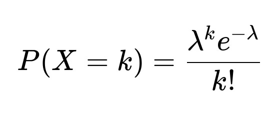
In this formula, X represents the random variable for the number of conversations started by a user in a single day, k is a non-negative integer representing the actual number of conversations observed, and lambda is the average number of conversations per user per day (the rate parameter).

Although actual usage might follow a distribution with heavier tails, the Poisson formula provides a conceptual baseline: if lambda is small, most users have zero or one conversation start per day, while a few might have higher counts. In reality, a platform could experience more dispersion than Poisson, leading to a handful of users having extremely high daily conversation counts.

Constructing an SQL Query for the Distribution

Below is an example SQL query that calculates how many conversations are created by each user on each day in 2020. For simplicity, let’s assume the table is named messages and it contains the following columns:

• sender_id: the ID of the user who initiates the message

• receiver_id: the ID of the user who receives the message

• message_date: the date (or datetime) the message was sent

• conversation_id: a unique identifier for each conversation thread

SELECT
    sender_id AS user_id,
    DATE(message_date) AS message_day,
    COUNT(DISTINCT conversation_id) AS total_conversations_created
FROM messages
WHERE YEAR(message_date) = 2020
GROUP BY sender_id, DATE(message_date);

Explanation of the query:

• sender_id identifies the user initiating the conversation.

• DATE(message_date) extracts just the date from any datetime value, helping group by day.

• COUNT(DISTINCT conversation_id) ensures we count the unique conversations initiated by that user on a particular day.

• The WHERE YEAR(message_date) = 2020 clause filters results to the year 2020.

If the goal is strictly the distribution of the daily counts (and not to see the breakdown by user), this result set can be further aggregated or processed to compute a histogram (for example, how many users started exactly 1 conversation on a given day, how many started 2, and so on).

Potential Follow-up Questions

How would you handle time zones or partial days in the data?

Time zone discrepancies can cause the same activity to be logged under different dates if the server’s time zone differs from the user’s local time. This might distort daily aggregates. One approach is to standardize all data to a single time zone (such as UTC) to avoid inconsistencies. Alternatively, you can store time zone information explicitly and perform localized aggregations if daily patterns by local time are required.

How could you detect anomalies or outliers in the distribution?

One approach is to compare daily conversation counts to historical averages. If a user who typically starts around five conversations per day suddenly jumps to hundreds of conversations, it might indicate spam or abnormal behavior. Statistical methods like standard deviation thresholds or robust approaches like median absolute deviation can help identify outliers.

Would a Poisson model always apply in this context?

Though the Poisson distribution is often the starting point for modeling count data, real user behavior can exhibit overdispersion (variance larger than the mean). In such cases, the negative binomial distribution or other heavy-tailed distributions could provide a better fit. This is especially true if there are large clusters of high-activity users or if the process generating the counts changes over time (e.g., new features introduced in the platform that boost engagement).

How might you visualize and interpret the distribution of daily conversation counts?

You could generate a histogram or a box plot of daily conversation counts per user. The histogram helps see how many users fall within each bin (like 0–5 conversations, 6–10, 11–20, etc.). A box plot can quickly reveal the median, quartiles, and potential outliers. Over time, you can track shifts in this distribution to understand growth or changes in engagement patterns.

What about considering the receiver’s perspective?

While this query focuses on conversations created by the sender, examining receiver data can illuminate responsiveness and any potential imbalance (for instance, many users receive messages from a small subset of senders). You could similarly group by receiver_id to analyze who is receiving the most messages, identify conversation clusters, or detect one-way message patterns.

How would you confirm data correctness?

You might compare the distribution with known usage benchmarks, check for unexpected spikes or zeros, and use logs or other usage metrics as cross-validation. Data quality checks might include verifying that conversation IDs are not duplicated in unexpected ways or ensuring there are no missing dates where the platform was presumably active.

How do you ensure this approach scales for large datasets?

For very large data, typical optimizations include:

• Partitioning the table by date or range to handle queries efficiently.

• Using indexes on sender_id and message_date.

• Employing a distributed data warehouse like BigQuery, Redshift, or Snowflake to process massive log data quickly.

• Building summary tables or materialized views on a daily basis to reduce the computational load when running historical analytics.

These strategies ensure that even if the messages table grows extremely large, daily aggregations remain manageable.

Below are additional follow-up questions

How might the presence of multiple user accounts or shared accounts influence the interpretation of daily conversation counts?

If some individuals have multiple accounts or if multiple individuals share a single account, daily conversation counts may be artificially inflated or deflated for each distinct user ID. For instance, a single person using multiple accounts could spread out conversations across these accounts, making each account appear less active. Conversely, if a single account is used by multiple people, that account’s statistics may show an unusually high message volume, masking the individual behaviors within.

From a data engineering perspective, one could:

• Track device or session fingerprints to link suspiciously overlapping accounts that might belong to a single user.

• Introduce sign-in checks to ensure an account is not shared in violation of terms of service.

• Use heuristics (e.g., identical IP ranges over time) to detect potentially linked accounts and label them for more nuanced analysis.

From an analytics perspective, you might handle multi-account users by collapsing all accounts linked to a single individual into a single “unified” user entry. This requires either a robust user identity system or an inference pipeline for merging suspiciously overlapping accounts. Failing to account for such factors can lead to misinterpreting real engagement levels and hamper the accuracy of downstream models or insights.

How do you account for seasonality or day-of-week effects in daily conversation counts?

Daily conversation volumes often exhibit strong seasonality (e.g., higher activity on weekends or specific holidays). Ignoring these patterns might cause misleading conclusions, such as attributing an expected dip on Mondays to platform issues rather than normal user behavior.

To incorporate seasonality:

• Segment data by day of the week or month and compare historical averages. For instance, analyze average Sunday conversation counts separately from weekdays.

• Use rolling averages or smoothing (e.g., a seven-day moving average) to account for within-week patterns.

• Employ time-series models (like SARIMA or Prophet) that explicitly model seasonality. This can help distinguish short-term anomalies from normal cyclical behavior.

Potential pitfalls include overlooking cultural differences in weekend days (e.g., Friday–Saturday in some regions vs. Saturday–Sunday in others) and ignoring big holidays or event-based spikes (New Year’s, major sports events, etc.). For truly global products, you might need region-specific modeling to reflect local holidays and cultural usage patterns.

If conversation_id can be reused or is not guaranteed to be unique, how might that impact your query?

When conversation_id is not strictly unique, using COUNT(DISTINCT conversation_id) might underestimate or overestimate the number of true conversation threads. For example, a messaging platform might reuse IDs or have collisions if the conversation_id is derived from non-random logic.

Potential mitigation strategies:

• Employ a composite key that includes both conversation_id and creation timestamp to ensure uniqueness.

• Investigate how conversation_id is generated and confirm the likelihood of collisions. If collisions are possible, track an additional field (like a session token or a creation timestamp) to help disambiguate.

• Validate integrity constraints in the data model to ensure collisions cannot happen inadvertently (e.g., by using a universally unique identifier (UUID)).

Failing to address this might lead to flawed distribution analysis, where it appears fewer or more conversations are initiated than actually occur. A thorough data validation step or ensuring the data schema enforces unique conversation identifiers is crucial.

How would you measure the impact of major product changes or marketing campaigns on these distributions?

Major product changes (such as a redesigned interface or new features like group chats) or marketing campaigns (like user acquisition drives) can significantly alter conversation patterns. Daily conversation counts might spike or shift to different user demographics. To analyze these impacts:

1. Set a Baseline Compare conversation counts for a suitable period (e.g., several weeks) before the campaign or product change to understand typical activity.

2. Mark Event Windows Explicitly record the start and end dates of the campaign or the release date of the new feature. Segment the data and compare the distribution before, during, and after the intervention.

3. Conduct Statistical Tests Use methods like t-tests or time-series intervention analysis (e.g., Causal Impact) to see if observed changes in conversation counts are statistically significant.

4. A/B Testing If possible, run an A/B test where a subset of users sees the new feature or campaign, and compare their conversation distributions to a control group.

A key pitfall is mistaking correlation for causation. There could be coincident external events (like seasonal holidays) that affect user behavior. By structuring the analysis carefully—ideally with controlled experimentation—you can more reliably attribute changes in conversation counts to the product update or campaign.

How do you handle the possibility of no messages or zero conversations on certain days for some users?

Zero-inflation (where many users have zero new conversations on a given day) is common. Simply ignoring days with zero messages can bias the analysis and obscure the overall distribution. Consider these steps:

1. Data Imputation Explicitly store records with count=0 to accurately represent inactive days.

2. Zero-Inflated Modeling Use statistical models that handle high frequencies of zeros (like zero-inflated Poisson or zero-inflated negative binomial distributions).

3. Analytical Implications Distinguish between users who are truly inactive (did not even log in) vs. those who logged in but did not initiate any conversation. This helps separate lack of engagement from presence but no conversation starts.

A pitfall is mislabeling user inactivity. For instance, if a user simply browses but doesn’t message, you might see zero conversation starts, but that doesn’t necessarily mean the user was absent from the platform. Identifying that nuance requires additional data sources (e.g., login logs or app usage events).

Could changes in user demographics affect the overall distribution of daily conversations?

Yes. If your user base grows in a new demographic or market with different messaging habits, the distribution might shift. For instance, younger users might send more frequent but shorter messages, whereas another demographic might prefer longer but fewer conversations.

1. Demographic Segmentation Break down conversation counts by user demographics (age group, region, language) to isolate differences.

2. Time-Window Analysis Compare distributions before and after known demographic shifts (e.g., after launching in a new country).

3. Population Weighting If analyzing a combined global distribution, consider weighting by the population of each demographic so that large or fast-growing groups don’t overshadow minority segments.

A subtle pitfall is attributing overall distribution changes to platform-wide factors when, in reality, they are driven by the influx of a new user segment. Recognizing that user composition changes is crucial for correct interpretation.

What if the platform introduces group conversations that involve more than two participants?

When group chats are introduced, a single “conversation” can involve multiple senders and receivers. Relying on a single sender_id and receiver_id might not be sufficient to measure how many new group threads a user initiates. One approach could be:

• Introduce a group flag in the messages table or track conversation participants in a separate table.

• Modify the query logic: for group conversations, consider the user who created the group thread as the “conversation initiator.” The other participants might be viewed as “invited” or “added” to that conversation.

Potential challenges include:

• Overcounting. If multiple participants send messages near the start of a group conversation, do we consider each as an initiator, or only the first user?

• Group vs. direct chat. Ensuring queries don’t mix counts from group chats with direct one-on-one chats unless intentionally desired.

Failure to differentiate one-on-one from group conversations could inflate or misrepresent the distribution of conversation counts for certain users, especially “super connectors” who frequently create group chats.

How would you integrate real-time analytics on conversation starts alongside batch processing for historical analysis?

For large-scale systems, you might have both real-time and batch data pipelines:

1. Real-time Stream Use technologies like Apache Kafka or AWS Kinesis for event streaming. Each message or conversation event is processed promptly, updating real-time dashboards that track the number of conversations initiated in the last minute/hour/day.

2. Batch Processing Use daily or hourly batch jobs with ETL tools (e.g., Spark or Flink) to build comprehensive historical views that include corrections (e.g., late-arriving data or updated conversation IDs).

The main pitfall is data consistency between real-time dashboards and batch-processed data. Real-time data might be incomplete or subject to minimal validation, whereas batch processes usually perform more checks and can incorporate late data. Ensuring alignment requires robust data governance, versioned data schemas, and reconciliation steps (i.e., verifying that the sum of incremental updates aligns with the final batch outcomes).

How do you detect and handle duplicate or replayed messages in the system?

Network issues or bugged clients can sometimes resend the same message multiple times, causing duplicated entries in the messages table. This can artificially inflate conversation counts:

1. De-duplication Strategies

   • Implement a unique key or checksum for each message at creation time, ensuring duplicates are recognized and discarded on ingestion.

   • Use an idempotent design in the messaging backend so repeated attempts to write the same message ID do not create new records.

2. Validation and Monitoring

   • Flag messages that arrive within an unrealistically short timespan with identical content or IDs.

   • Set up anomaly detection to alert if the daily conversation volume spikes in a suspiciously short interval.

If duplicates slip through, your aggregated metrics (like the total number of conversations initiated per day) may be overstated. Addressing this requires consistent data cleaning and robust system design to avoid polluting downstream analytics.

How would you accommodate newly introduced user or message metadata (e.g., message topic, device type, or usage context) in your existing analysis?

Adding new metadata might mean altering how you define or group conversations. For example, if messages now include a “topic” field, you can slice your distribution by conversation topic to understand which topics garner the most daily starts.

Considerations include:

• Schema Evolution Update the schema in your data warehouse or lake to incorporate new columns or dimension tables (e.g., a topics dimension).

• Migration and Backward Compatibility Messages prior to the new metadata might have null or default values for the new field, so your analytics need to handle incomplete data gracefully.

• Revisiting Business Logic If conversation_id is partially determined by the “topic” or device type, ensure your aggregator query still accurately reflects conversation uniqueness.

Pitfalls: mixing old and new data can lead to inconsistent analyses if your definitions change midstream. A robust data engineering practice is to track changes to the data model and apply versioning or transformations that unify older records with newly enhanced records.

How would you handle queries that need to differentiate between “created” vs. “first message sent” for a conversation?

Sometimes “conversation creation” is distinct from the first message. You might have a system that marks a new conversation object in the database when a user starts drafting but hasn’t yet sent a message. Alternatively, the conversation object might only be created upon sending the first message. These nuances affect how you count “conversations created.”

1. Clear Definition Align on whether “creation” means the user officially starts a conversation object or the first message is actually sent.

2. Data Model Audit Ensure you know whether the platform’s data model includes a placeholder conversation record or only generates conversation objects when a first message is sent.

3. Measure Delays If there’s a potential time gap between conversation creation and the first message, you might see the conversation object date differ from the message date.

A pitfall is double counting or undercounting if the logic for conversation creation vs. first message is not consistent. If you have multiple states for conversations (draft, active, archived), ensuring consistent usage of each state is key for analytics correctness.