ML Interview Q Series: What is Data Binning? When would you use Equal Frequency Binning and when do you use Equal Width Binning?

📚 Browse the full ML Interview series here.

Comprehensive Explanation

Data binning (also known as data discretization) is a technique where continuous or large-scale numeric data is grouped into intervals called “bins.” Instead of each individual numeric value, we store or analyze the bin index or category. This can help reduce noise, prevent overfitting, and allow for simpler models or insights, especially when dealing with data visualization or certain ML algorithms that benefit from categorical features.

Equal Width Binning

Equal width binning is when you divide the data range into bins of equal size. To do this, you typically find the minimum and maximum of the data, choose how many bins you want, and then calculate the bin width. A core formula often used for computing the bin width in equal width binning is:

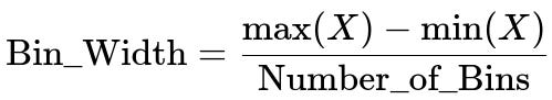
Here, max(X) and min(X) are the maximum and minimum values in your dataset X, and Number_of_Bins is the total number of bins you decide to create. Each bin covers a specific subrange of the data with the same fixed width.

Equal width binning is typically used when you want consistent, fixed-size intervals across your entire range of data. It can be helpful in certain scenarios:

• You want interpretability of intervals in a uniform manner. • Your data range is nicely distributed (for example, almost uniform or near-uniform distributions). • You prefer the bin boundaries to be consistent (like 0–10, 10–20, 20–30, etc.).

A key downside is that if the data is highly skewed, some bins might contain many data points while others might be almost empty, leading to an unbalanced representation.

Equal Frequency Binning

Equal frequency binning divides the data such that each bin contains (approximately) the same number of data points. Unlike equal width binning, the interval widths will vary because the data distribution will affect where the boundaries fall. In practice, you might:

• Sort the data points. • Partition the sorted data into contiguous subsets, each holding roughly the same count of data points.

Equal frequency binning is often used when you want to ensure that each bin is equally represented in terms of data points. It can be particularly useful:

• If your data is skewed and you want to avoid empty or overloaded bins. • If you need balanced categories for specific downstream tasks.

However, because the bin boundaries depend on the distribution of the data, you lose uniformity in the actual numeric ranges. Interpreting the bin boundaries might be less straightforward, and small changes in data can shift boundaries dramatically if the data near the thresholds is dense.

Practical Example in Python

Below is a small example using pandas, demonstrating how to apply equal width binning with cut and equal frequency binning with qcut:

import pandas as pd

# Sample numeric data
data = [1, 2, 3, 5, 7, 10, 15, 16, 18, 30, 45, 46, 47, 100]
df = pd.DataFrame({'value': data})

# Equal Width Binning: 3 bins
df['equal_width_bin'] = pd.cut(df['value'], bins=3, labels=False)

# Equal Frequency Binning: 3 bins
df['equal_freq_bin'] = pd.qcut(df['value'], q=3, labels=False)

print(df)

In this snippet:

• pd.cut with bins=3 divides the entire numeric range from min(data) to max(data) into 3 equal-width intervals. • pd.qcut with q=3 divides the data into 3 bins where each bin has an equal fraction (about one-third) of the data points.

Follow-up Questions

Why might data binning help reduce overfitting in a model?

Binning transforms continuous variables into discrete categories. This discretization can reduce the model’s sensitivity to minor fluctuations or noise in continuous inputs. Many sophisticated models (like decision trees) can overfit if there are too many fine-grained splits. By consolidating ranges of values into bins, the model gains a smoother representation of the input space, often leading to better generalization. However, there is a trade-off because too few bins can lose important information.

How do we choose the right number of bins?

Choosing the number of bins is often guided by domain knowledge, empirical experimentation, or rules of thumb (for example, the Sturges or Freedman-Diaconis rules in histograms). An analyst might:

• Use cross-validation performance metrics to compare different bin counts. • Take into account the total number of data points (too many bins might lead to very sparse bins, too few might lump distinct values together). • Consider domain-specific boundaries or business context (like age group bins in medical data).

Are there any downsides to data binning?

While binning can be beneficial, there are some caveats:

• Potential loss of information: Subtle variations within a bin cannot be distinguished. • Boundary issues: Slight changes in data close to bin boundaries can lead to large category changes. • Possibly arbitrary cut points: Equal width binning might be unbalanced if the data is skewed, and equal frequency binning might have inconsistent interval widths that complicate interpretation.

What if my data has outliers?

Outliers can affect the min and max in equal width binning, making most bins very narrow for the majority of the data while one bin covers a huge range to accommodate outliers. Equal frequency binning can also be impacted if the outliers appear close together in a small region, affecting the distribution of your bins. Common strategies:

• Clip or transform outliers before binning. • Use binning methods specifically designed for outlier-robustness (e.g., ignoring extreme percentiles). • Consider a hybrid approach that uses quantile-based splits but adds a special bin for extreme values.

Are there scenarios where I should avoid binning?

You might avoid binning if:

• The continuous nature of the data is critical for the model. • You have a sufficiently large dataset and a model that can handle continuous features well (like gradient boosted trees or neural networks). • You require high precision or subtle numeric distinctions (binning can mask nuances).

In many modern machine learning practices, especially with large datasets and non-linear models, binning is not always essential. Still, it remains a powerful technique in specific contexts, especially when dealing with smaller samples, using certain classical algorithms, or requiring interpretability.

Below are additional follow-up questions

How do you handle missing values when applying data binning?

Missing values pose a subtle challenge for binning because a missing value does not inherently fall into any numeric range. In practice, you can address this in multiple ways. One common approach is to create an additional bin specifically for missing values. This isolates missing data so that the model can learn any unique patterns associated with the absence of a value. If you simply drop missing records, you may lose valuable information about why those entries were missing in the first place. Alternatively, if the proportion of missing data is small, you might impute the values based on domain knowledge or statistical methods such as mean or median imputation. However, imputation before binning could bias the distribution, particularly if your data is skewed or if the missingness is not random. Creating a separate bin for missing values maintains a clear distinction between actual numeric ranges and absence of data, which can be critical in tasks that rely on detecting unusual or systemic missingness patterns.

Can data binning introduce artificial patterns or discontinuities in the data?

Binning converts continuous data into discrete intervals, which inherently introduces boundaries. A single data point just below a bin edge versus one just above that edge might be placed into two distinct categories even though their values differ only marginally. This can lead to abrupt transitions in your features, effectively creating artificial “steps” in the feature space. Models that rely on these newly introduced categorical edges may pick up on differences that are not truly meaningful in the real numeric sense. Additionally, if the bins are not chosen carefully (for example, uniform bins in a heavily skewed distribution), you may inadvertently concentrate most of the data in a small number of bins while underpopulating other bins, making the model sensitive to those arbitrary splits. This discontinuity effect is one of the reasons why binning can sometimes reduce interpretability when dealing with borderline data points or when the actual numeric scale holds important incremental relationships.

What happens if the data distribution changes over time (concept drift) and we have already applied fixed binning?

Concept drift occurs when the statistical properties of the target variable or features change over time. If you have applied binning based on a historical distribution, and the underlying distribution shifts, your previously defined bins may no longer be valid or balanced. For example, if your data starts to occupy ranges that were previously rare, you might end up with bins that are poorly suited for the new data distribution. In such a case, you would need to either dynamically update your bin definitions or periodically re-calculate them from the latest data. However, dynamically updating the bins can disrupt model consistency, especially if historical predictions used older bin definitions. This can complicate monitoring and understanding long-term metrics. A common solution is to adopt a window-based or incremental binning strategy, recalculating bins at set intervals or upon detection of distributional shifts. In streaming or real-time systems, you might implement adaptive discretization methods that adjust bin boundaries as new data arrives.

How can binning affect partial dependence analysis or feature importance in certain models?

Partial dependence plots and feature importance metrics often assume a smooth relationship between numeric features and model outputs. When you convert a continuous feature into bins, each bin becomes a nominal category, and the model may treat these categories as distinct, non-ordinal values. This can cause the partial dependence relationship to appear stepwise, which may obscure the underlying continuous relationship. Moreover, feature importance algorithms (such as impurity-based importance in decision trees) might assign different importances to bins that dominate splits, making it harder to interpret the genuine numeric influence of the original feature. If feature interpretability is crucial, you may consider alternative methods such as monotonic binning (where bin edges follow an increasing or decreasing pattern based on domain constraints) or binning only when it genuinely improves model stability. Another strategy is to keep both the binned and continuous versions of the feature, then compare how the model uses each, though this can introduce multicollinearity issues if not handled carefully.

Are there any sophisticated binning techniques that adapt to the data beyond simple equal width or equal frequency methods?

There are more advanced methods of binning that dynamically adjust to the nature of the data. Decision-tree-based discretization is one such technique, where a decision tree is trained on a single feature (and perhaps the target). The tree’s splits then define the bin boundaries in a way that is potentially more aligned with predicting the outcome. This method can yield more predictive bins but can also risk overfitting if not regularized properly. Another approach is clustering-based binning, where you apply a clustering algorithm (like k-means) to one-dimensional data and treat each cluster as a bin. This can be particularly useful if the data shows distinct modes or natural groupings. However, both these approaches can be more computationally complex and might overfit or create unintuitive bins. Additionally, you can use quantile-based binning that ignores extreme tails by focusing on selected percentiles, which can help mitigate the effect of outliers while ensuring that bin distribution remains balanced.

How do you combine data binning with other feature engineering techniques without losing too much information?

When combining binning with more advanced feature engineering, a careful balance is required. If you have powerful continuous transformations—such as polynomial terms, logarithmic transformations, or learned embeddings in neural networks—binning might negate those benefits by coarsening the resolution of your features. One best practice is to generate both binned and un-binned versions of key features, then let your model’s feature selection or regularization methods decide which representation is more predictive. You could also use binning as a starting step for interpretability and for certain models that rely on categorical data (like Naive Bayes or certain rule-based methods). Furthermore, you can incorporate domain-knowledge-driven bin boundaries that combine the strengths of both approaches. For example, if a domain standard lumps ages into certain medical risk categories, you might preserve those categories while still providing the raw age to the model. This way, you capture domain knowledge without sacrificing the fine-grained detail that might be crucial to more sophisticated modeling approaches.