
ML Interview Q Series: What is the difference between Objective function, Cost function and Loss function

📚 Browse the full ML Interview series here.
Comprehensive Explanation
Objective function, cost function, and loss function are closely related concepts in machine learning optimization, yet they have some nuanced differences in how they are used and what they represent.
Objective Function
The objective function is the broader term for the function we want to optimize (maximize or minimize) during training. It might include not just the measure of prediction error but also other terms (for instance, regularization terms). In many contexts, the objective function is the overall mathematical expression that drives model training. Its goal could be:
• Minimizing error on the training set. • Incorporating penalties to reduce overfitting (e.g., L2 regularization). • Maximizing likelihood or posterior probability in Bayesian settings.
Sometimes, people use the term "objective function" interchangeably with "cost function" or "loss function," but strictly speaking, the objective function can include more than just the average or total error. For instance, it might combine the sum of the errors and a regularization penalty.
Cost Function
The cost function is typically the aggregate (often the mean or sum) of the discrepancies between predictions and ground truth across the entire training set. You can think of the cost function as an average or sum of losses over all data points. Many people also refer to it as the training error. Minimizing this cost function is usually the objective of the training process (although strictly speaking, with regularization we often add more terms into the objective).
A common example of a cost function for regression problems is the Mean Squared Error (MSE) across N samples:
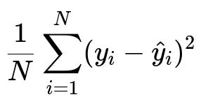
where y_i is the true target for the i-th data point, and \hat{y}_i is the model’s prediction for the same data point. N is the total number of data points in the training set. This formula represents the average of the squared difference between predicted and actual values. Minimizing this encourages the model to produce predictions that are close to the actual data.
In many classification settings, the cost function could be the average cross-entropy, which is again a sum or mean of the individual losses for each data point.
Loss Function
The loss function usually denotes the error for a single training example (or sometimes for a single batch). It quantifies how far off a model’s prediction is from the true value for that single data point. For instance, in a regression setting, the squared loss for a single data point might be (y_i - \hat{y}_i)^2. The cost function, on the other hand, often takes the average (or sum) of these losses over all training samples.
In many references, "cost function" and "loss function" are used nearly interchangeably. However, some texts strictly define "loss function" at the individual sample level and "cost function" as an aggregated measure over the entire dataset. In practice, this distinction is sometimes blurred, but it’s beneficial to be aware of the nuance.
Why They Matter
Understanding the difference ensures clarity in discussions about optimization. For example:
• When implementing gradient-based methods, at each training step you often compute the loss for a batch or a single example, then update parameters. • Over the course of an epoch, you compute the aggregate cost to see how the model performs on all training samples. • Your ultimate objective function might also include a regularization term, which shapes the final parameter solution.
Hence, you might see statements like: “We are minimizing the cost function J, which is the sum of the individual losses plus a regularization term.” That cost function is effectively your objective function, but the pure “loss function” (e.g. MSE or cross-entropy) might not necessarily include the regularization part.
Follow-up Question 1
What are some examples of loss functions for classification and how do they relate to the cost function?
When dealing with classification, common loss functions include cross-entropy loss (also called log loss) and hinge loss. The cross-entropy loss for a single binary classification example with label y in {0, 1} and predicted probability p is often given by -[y log(p) + (1-y) log(1 - p)]. For multiple classes, this generalizes to the categorical cross-entropy. The cost function usually aggregates these individual losses (e.g., via a sum or mean over the entire dataset). In code, this might look like summing the cross-entropy over all samples and then dividing by the total number of samples.
Follow-up Question 2
How does the inclusion of a regularization term in the objective function affect model training?
Regularization modifies the objective function by adding a penalty term that discourages overly large or overly complex parameter values. For instance, L2 regularization adds a penalty proportional to the sum of squares of the weights. This leads the optimization to trade off between minimizing the model’s training error and keeping parameters small. The net effect is better generalization and reduced overfitting. Concretely, your objective function might be cost_function + lambda * regularization_term, which effectively modifies the gradients and encourages simpler solutions.
Follow-up Question 3
How do you select an appropriate loss or cost function for different tasks?
The choice depends on the nature of the problem and the type of output:
• Regression: Mean Squared Error or Mean Absolute Error are commonly used. MSE penalizes large deviations more heavily, while MAE is more robust to outliers. • Classification: Cross-entropy is typically used, though hinge loss (for SVMs) and focal loss (for imbalanced problems) are also popular. • Ranking / Metric-specific tasks: You might use pairwise ranking losses or specialized metrics like ROC-AUC–based approximations if the final goal is to optimize a certain ranking metric.
The cost function usually aggregates your chosen loss function over your dataset.
Follow-up Question 4
What if a cost function is non-differentiable? How do we optimize it?
Non-differentiability can arise if the cost or loss involves absolute values, piecewise functions, or other operations that are not smooth. Possible strategies include:
• Using sub-gradients, which generalize the concept of gradients to non-differentiable functions. • Employing gradient-free methods like evolutionary algorithms or certain metaheuristics. • Approximating the non-differentiable function by a differentiable surrogate that is easier to optimize.
In deep learning frameworks, certain non-differentiable components (e.g. ReLU at zero) are still handled effectively because of sub-gradient rules for piecewise linear functions.
Follow-up Question 5
When do we typically use squared error vs. cross-entropy in neural networks?
Squared error is used primarily in regression tasks where output is a continuous value. For classification tasks, cross-entropy is often preferred since it directly measures the difference between the predicted probability distribution and the target distribution, leading to smoother gradients and faster convergence for classification. In some rare cases, one might still experiment with squared error for classification, but it’s less conventional compared to cross-entropy.
Follow-up Question 6
Are there scenarios where the terms "cost function," "loss function," and "objective function" are used interchangeably?
Yes. In many practical machine learning contexts, you will see these terms used interchangeably because many textbooks and frameworks do not strictly enforce the differences. Practitioners commonly say “loss function” when they really mean the aggregated form or the entire objective. However, it is valuable to understand the precise definitions to avoid confusion:
• The loss function often refers to the measure of error at an individual sample level. • The cost function frequently denotes the aggregate (sum or average) loss over the entire training set. • The objective function is the all-encompassing function to be optimized, which may include the cost (sum of losses) plus additional terms (like regularization).
The usage in everyday conversation may blur these lines, but in formal contexts (e.g., certain research papers or advanced textbooks), the distinction can be quite important.
Below are additional follow-up questions
Follow-up Question 7
What happens if our chosen cost function is poorly aligned with our real-world goal?
When we define a cost function, we assume it captures the real-world metric we care about. However, in practice, mismatches can occur. For example, in a medical context, using Mean Squared Error as a cost function for a regression model might not reflect the actual cost of different magnitudes of errors. A small error could be far less critical in some cases compared to a large error that leads to a misdiagnosis.
Pitfalls arise if the cost function overemphasizes certain errors or underemphasizes others. This can lead the model to optimize for something that doesn't align with the business or clinical objective. To address this, practitioners may:
• Incorporate domain-specific cost weighting. For example, penalize large errors more heavily if they have dire consequences. • Shift from standard regression metrics to more specialized error metrics, such as quantile-based metrics (if underestimation or overestimation has different costs). • Integrate additional constraints to reflect domain requirements better.
Real-world scenarios often demand iterative refinement of the cost function once a mismatch is observed.
Follow-up Question 8
Can we combine multiple cost functions or losses into a single objective function, and how does that work in practice?
Yes, multi-objective optimization is sometimes required when there are multiple aspects of a problem we wish to optimize simultaneously. For example, we might want to minimize both MSE (to ensure accuracy) and the L1 norm of the parameters (to enforce sparsity). A common approach is to form a weighted sum of each cost function:
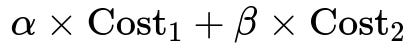
In this expression, alpha and beta are hyperparameters controlling the relative importance of each cost. Practitioners usually tune these hyperparameters to find an acceptable trade-off. Pitfalls include:
• Overemphasis on one term at the expense of others. • Difficulty in selecting the weighting coefficients. • Potential conflicts between objectives where improving one metric may worsen another.
When dealing with more than two objectives, advanced techniques like Pareto optimization may be used to find an entire set of optimal trade-offs.
Follow-up Question 9
How do we handle constraints (like fairness or specific performance thresholds) within an objective function?
In certain real-world applications, it’s not enough to minimize a cost function; we must also maintain specific constraints. These constraints might be legal or ethical, especially in sensitive domains such as lending, insurance, or hiring. A few ways to integrate constraints include:
• Constrained Optimization: Formally incorporate constraints g(x) <= 0 into the optimization. Solvers like constrained gradient methods can handle these. • Penalty Methods: Add a large penalty term whenever constraints are violated, encouraging solutions that satisfy the constraint. • Post-hoc Adjustments: Train with a standard objective first, then adjust predictions to meet constraints. This can be less efficient since you might degrade performance unnecessarily.
Pitfalls arise if constraints conflict with the primary objective or if penalty terms are not tuned correctly. In fairness contexts, for example, you might find that a strong constraint ensures equitable predictions for all subgroups, but overall model accuracy declines, requiring careful compromise.
Follow-up Question 10
What is the difference between training, validation, and test cost (or loss), and why does it matter?
• Training Cost/Loss: This is the quantity directly minimized during model training. If it decreases over time, the model is learning to fit the training data better. • Validation Cost/Loss: Computed on a separate validation set. It indicates how well the model generalizes beyond the training data. It is crucial for hyperparameter tuning. • Test Cost/Loss: Calculated on a completely held-out dataset that played no role in model selection or tuning. It provides the most unbiased estimate of generalization.
Pitfalls include:
• Overfitting the training data, causing the training loss to be low, but validation and test losses to be high. • Over-tuning hyperparameters on the validation set, which can subtly leak information about the validation set and lead to an optimistic estimate of performance. • Distribution shifts between training and validation/test sets, making the validation/test losses unreliable indicators of real-world performance.
Follow-up Question 11
How do we handle label noise or outliers in the training data when defining a cost function?
Label noise or outliers can heavily bias common losses (like MSE) because squared errors grow rapidly with large deviations. Methods to address this include:
• Robust Loss Functions: Examples like Huber loss or Tukey’s biweight loss reduce the influence of outliers. • Data Cleaning: If feasible, identify and remove or correct erroneous data points before training. • Regularization: Strong regularization (L1 or L2) sometimes mitigates the model’s tendency to fit outliers exactly. • Iterative Refinement: After an initial model fit, evaluate high-error samples to detect potential mislabels.
A pitfall is that removing data might introduce biases if certain subpopulations are consistently flagged as “outliers.” Also, switching to a robust loss can sometimes reduce overall accuracy if the “outliers” were actually valid but complex examples.
Follow-up Question 12
How do we optimize non-differentiable metrics, like Precision/Recall or F1 score, as our main objective?
Common classification metrics such as Precision, Recall, and F1 score are not differentiable with respect to model parameters, posing challenges for gradient-based optimization. Approaches include:
• Surrogate Losses: Use cross-entropy or hinge loss as a differentiable proxy while monitoring the non-differentiable metric as an evaluation measure. • Approximate Differentiation: Some advanced techniques approximate the gradient of these metrics. This can be computationally expensive and less stable than using standard differentiable losses. • Reinforcement Learning or Evolutionary Algorithms: These approaches can optimize non-differentiable objectives but are typically slower and more complex than direct gradient-based methods.
A pitfall is that optimizing a surrogate loss does not guarantee optimal F1 if the data distribution or class imbalance is significant. There is always a risk of mismatch between your surrogate loss and your real evaluation metric.
Follow-up Question 13
What is the impact of high-dimensional parameter spaces on objective functions, and how can this complicate training?
In high-dimensional spaces (common in deep learning), the objective landscape can have many local minima, saddle points, and plateaus. Some practical challenges include:
• Many Local Optima: Though modern neural networks often find reasonably good minima, there could be many regions in parameter space where the gradient is small or where the function is only locally optimal. • Saddle Points and Plateaus: Large flat regions or plateaus make it harder for gradient-based methods to make progress. • Vanishing/Exploding Gradients: In deep networks, gradients can become extremely small or excessively large, slowing or destabilizing training.
To mitigate these issues, techniques include careful initialization, adaptive optimizers (Adam, RMSProp), skip connections (in deep architectures), and batch normalization.
Follow-up Question 14
How do advanced optimization techniques (like Adam, RMSProp, or second-order methods) interact with the choice of cost or loss function?
Advanced optimizers adapt the learning rate or incorporate second-order information about the loss surface. This can affect how quickly the model converges and how stable training is:
• Adam: Uses moving averages of gradients and squared gradients, making it well-suited for sparse gradients or rapidly changing loss surfaces. It can adapt learning rates per parameter. • RMSProp: Maintains an exponentially weighted moving average of squared gradients, helping to control the step size for each parameter. • Second-order methods: Attempt to leverage the Hessian matrix or its approximations. They can converge in fewer steps if the cost function is well-defined, but computational overhead is significant for large models.
Pitfalls include choosing improper hyperparameters (learning rate, decay rates, etc.) that cause oscillations or slow convergence. Moreover, some optimizers may overshoot if the cost function changes dramatically in certain regions, especially if the gradient estimates are noisy.