
ML Interview Q Series: What is the probability mass function of total sixes when rolling a die based on the first roll?
Browse all the Probability Interview Questions here.
Short Compact solution
Consider the first roll’s outcome to be j. This occurs with probability 1/6 for j = 1, 2, …, 6. If 1 <= j <= 5, the probability of getting k total sixes (counting the first roll) is the binomial probability (j choose k) (1/6)^k (5/6)^(j-k), where (j choose k) is taken to be 0 if k>j. If j=6, then we already have one six from the first roll, and we need k-1 sixes from the next 6 rolls. That probability is (6 choose (k-1)) (1/6)^(k-1) (5/6)^(6 - (k-1)). By summing over j from 1 to 5 and adding the contribution from j=6, each weighted by 1/6, we get:
For k = 1, 2, …, 7:
Numerically, these probabilities are approximately:
P(X=0) = 0.4984
P(X=1) = 0.3190
P(X=2) = 0.1293
P(X=3) = 0.0422
P(X=4) = 0.0096
P(X=5) = 0.0014
P(X=6) ≈ 3.57×10^-6
P(X=7) ≈ 1/6^7
Comprehensive Explanation
Defining the random variables
Let N be the outcome of the first roll of a fair, six-sided die. So N can be 1, 2, 3, 4, 5, or 6 with probability 1/6 each. Then, given N=j, we roll the die j more times. We define X to be the total number of sixes observed: one six may come from the initial roll if it shows a 6, plus however many sixes appear in the subsequent j rolls.
Hence:
If j in {1, 2, …, 5}, we have a total of j+1 rolls, but to count the total number of sixes X, the first roll might or might not be a six.
If j=6, we have 1 (the first roll, which is definitely a six) plus 6 additional rolls, so 7 rolls in total. We already know that the first roll is a six in this scenario, so the remaining 6 rolls determine how many more sixes appear (k-1 more sixes if we want a total of k).
Using conditional probability
We use the law of total probability to write P(X=k) as a sum over all possible values of N:
P(X = k) = sum over j from 1 to 6 of [P(X = k | N = j) * P(N = j)].
Since the die is fair, P(N = j) = 1/6. Thus,
P(X = k) = (1/6) * sum over j from 1 to 6 of P(X = k | N = j).
When 1 <= j <= 5
If the first roll is j in [1..5], then among these j rolls, we want k sixes total. This can happen only if the first roll is a six and some subset of the next (j-1) rolls are sixes, or if the first roll is not a six but some subset of the j subsequent rolls are sixes, etc. However, it is simpler to see it as a single binomial draw of size j on the event of "roll is six," with probability 1/6 per roll, ignoring the first roll or counting it among the j. The standard binomial formula emerges:
Probability = (j choose k) (1/6)^k (5/6)^(j-k),
assuming (j choose k) = 0 if k>j. This formula lumps the first roll with the subsequent j-1 rolls for counting the total k sixes among j independent Bernoulli(1/6) trials.
When j = 6
If the first roll is a 6, we already have 1 success. Now we roll the die 6 more times. So to get k total sixes, we need (k-1) additional sixes from these 6 rolls. The probability of that event is:
(6 choose (k-1)) (1/6)^(k-1) (5/6)^(6 - (k-1)).
Summation and final pmf
Putting the two cases together and summing over all j:
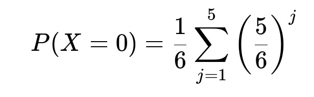
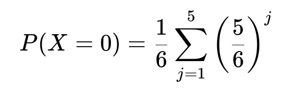
For k=0:
We cannot have j=6 because that guarantees at least one six. So j must be in {1..5}, and we get 0 sixes if all j rolls are not six. That is (5/6)^j for each j. Weighted by 1/6:
For k>=1 (up to k=7, because 7 sixes is the maximum if the first roll is 6 and then all subsequent 6 rolls are also sixes):
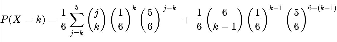
The first summation covers j from k to 5 for the standard binomial scenario (1 <= j <= 5).
The second term covers j=6, where we have the first roll already a success and look for k-1 successes in the next 6 rolls.
The notation (j choose k) = 0 if k > j ensures we do not incorrectly count impossible events.
Potential edge cases
k = 0: This can only occur if j is in {1..5} and none of those j rolls nor the first roll are sixes.
k = 7: This occurs if and only if the first roll is 6 and all 6 additional rolls are sixes, which has a small probability: (1/6)(1/6)^6 = 1/6^7.
Numerical values
One may compute these probabilities directly and confirm they sum to 1. Numerically they are (approximately):
P(X=0) = 0.4984
P(X=1) = 0.3190
P(X=2) = 0.1293
P(X=3) = 0.0422
P(X=4) = 0.0096
P(X=5) = 0.0014
P(X=6) ≈ 3.57×10^-6
P(X=7) ≈ 1/6^7
Below is a quick Python snippet that demonstrates how to compute this pmf programmatically.
import math

def pmf_X(k):
    # Probability that first roll is j
    # For j in [1..6], each has probability 1/6
    if k == 0:
        # Special case
        total_prob = 0.0
        for j in range(1, 6):  # j=1..5
            total_prob += ( (5/6)**j )
        return (1/6) * total_prob
    else:
        total_prob = 0.0
        for j in range(k, 6):  # j= k..5
            # binomial(j, k) * (1/6)^k * (5/6)^(j-k)
            # but watch if k>j, this automatically is 0
            if k <= j:
                comb_jk = math.comb(j, k)
                total_prob += comb_jk * (1/6)**k * (5/6)**(j-k)
        # j=6 case:
        # need k-1 successes in next 6 rolls
        if k-1 <= 6 and k-1 >= 0:
            comb_6_k_1 = math.comb(6, k-1)
            total_prob += comb_6_k_1 * (1/6)**(k-1) * (5/6)**(6 - (k-1))
        return (1/6) * total_prob

# Print out probabilities for k=0..7
for k in range(8):
    print(k, pmf_X(k))
Possible Follow-Up Questions
What is the expected value E[X]?
To find the expectation, we can use the law of total expectation. Let X be the total number of sixes, N be the outcome of the first roll.
E[X] = E[E[X | N]].
E[X | N=j] = expected number of sixes in the first roll plus j subsequent rolls. The first roll has a 1/6 chance of being six, so its expectation is 1/6. The next j rolls each has expectation 1/6. So E[X | N=j] = (1/6) + j*(1/6) = (1 + j)/6.
Since N is equally likely to be 1, 2, 3, 4, 5, or 6, we have E[N] = 3.5. Thus:
E[X] = E[ (1+N)/6 ] = (1/6) E[1+N] = (1/6)(1 + E[N]) = (1/6)(1 + 3.5) = 4.5/6 = 0.75.
Hence, E[X] = 0.75.
Could we use a probability-generating function approach?
Yes. We could define G_X(t) = E[t^X]. By conditioning on N, we derive G_X(t) = (1/6)*sum_{j=1..5} E[t^X | N=j] + (1/6)*E[t^X | N=6]. For j in [1..5], the generating function for the number of sixes among j i.i.d. Bernoulli(1/6) trials is ( (5/6 + (1/6)t )^j ), and we would need to handle j=6 by factoring in the guaranteed six. This is more elaborate, but the final pmf we derived is typically the simpler route.
How would we verify this pmf sums to 1?
We can sum over k = 0..7 the probabilities P(X=k) and verify we get 1. Because the maximum number of sixes is 7 (if first roll is 6, plus the next 6 are all sixes). Any other event yields fewer than 7 sixes. A quick Python check (like the snippet above) or a manual summation confirms correctness.
Could the range of X be different?
In principle, X cannot exceed 7 because:
We have 1 roll for the first throw.
If it shows 6, then we do 6 more rolls. Hence total number of rolls is at most 7, so X cannot be larger than 7. And obviously X cannot be negative, so the support is X in {0,1,2,3,4,5,6,7}.
What if we needed the distribution of N + X (i.e., total number of rolls plus total number of sixes)?
This is a different question but highlights how random sample size can combine with counting the number of “successes.” We would carefully define a new random variable Y = N + X. Then we would do a similar conditioning approach or a bivariate approach. Such questions often appear in advanced probability topics on random sums of random variables.
All these considerations demonstrate the fundamental approach of conditioning on the first roll, enumerating all possible outcomes, and carefully accounting for the binomial probabilities in the subsequent rolls.
Below are additional follow-up questions
1) Could we compute Var(X), the variance of X, using the law of total variance?
Answer Yes. One powerful way to compute Var(X) is to use the law of total variance, which states:
Var(X) = E[Var(X | N)] + Var(E[X | N]).
Recall that N is the outcome of the first roll, taking values 1 through 6 with probability 1/6 each. We already know the following:
E[X | N=j] = (1/6) + (j/6). This is because the first roll has a 1/6 chance of being a six, and the j subsequent rolls also each have a 1/6 chance of being six.
Var(X | N=j] is the variance of the total number of sixes among 1+j rolls, each having probability 1/6 of being a six. For a Binomial random variable with parameters n and p, the variance is n p (1-p). So if the first roll is j (in [1..5]), we effectively have a Binomial(j, 1/6), except we are including the first roll in that binomial count. Concretely:
When j in {1..5}, X|N=j ~ Binomial(j, 1/6). Then Var(X | N=j) = j*(1/6)*(5/6).
When j=6, the first roll is guaranteed to be a six plus a Binomial(6, 1/6) for the next six rolls. So in total, X | (N=6) is 1 + Binomial(6, 1/6). The variance of (1 + Binomial(6, 1/6)) equals the variance of Binomial(6, 1/6), which is 6*(1/6)*(5/6).
Hence, for j=1..5, Var(X|N=j) = j*(1/6)(5/6). For j=6, Var(X|N=6) = 6(1/6)*(5/6).
Step 1: Compute E[Var(X | N)]. We average Var(X | N=j) over j=1..6:
E[Var(X | N)] = (1/6) * [ sum_{j=1..5} ( j*(1/6)(5/6) ) + 6(1/6)*(5/6 ) ].
Step 2: Compute Var(E[X | N]). We have E[X | N=j] = (1 + j)/6. Thus,
Var(E[X | N]) = Var( (1 + N)/6 ) = (1/36) * Var(1 + N) = (1/36)*Var(N).
Since N is uniform on {1,2,3,4,5,6}, its variance is (6^2 - 1)/12 = 35/12, so Var(N) = 35/12. Therefore,
Var(E[X | N]) = (1/36)*(35/12) = 35/(432).
Step 3: Sum them up. Var(X) = E[Var(X | N)] + Var(E[X | N]).
This gives the exact variance. A common pitfall is to forget that the first roll might already be a six when N=6, so you should not treat it purely as a Binomial(n+1, 1/6) in that scenario but rather 1 plus Binomial(6, 1/6). However, since Var(1 + Y) = Var(Y), it often does not change the variance from the simple binomial expression aside from ensuring you properly handle E[X | N=6] in the second term.
This approach elegantly avoids confusion by always working inside the conditional distribution and then using the law of total variance.
2) How do we find Cov(X, N)?
Answer The covariance of X and N is given by
Cov(X, N) = E[X * N] - E[X] * E[N].
We know:
E[N] = 3.5, because N is uniform on {1..6}.
E[X] = 0.75, as found previously using E[X|N=j] = (1 + j)/6 and then averaging over j.
To get E[X * N], we use the fact:
E[XN] = E[ E[XN | N] ] = sum_{j=1..6} [ E[X*N | N=j ] * P(N=j) ].
But X*N = N * X, so, given N=j,
E[X*N | N=j] = j * E[X | N=j].
Since E[X | N=j] = (1 + j)/6, then
E[X*N | N=j] = j * [ (1 + j)/6 ].
Each j occurs with probability 1/6, so
E[X*N] = (1/6) * sum_{j=1..6} j * (1 + j)/6 = (1/36) * sum_{j=1..6} [ j(1 + j) ].
We compute sum_{j=1..6} [ j(1 + j) ] = sum_{j=1..6}[ j + j^2 ] = 21 + 91 = 112. Hence,
E[X*N] = (1/36)*112 = 112/36 = 28/9.
Finally,
Cov(X, N) = (28/9) - (0.75)(3.5).
Since 0.75 * 3.5 = 2.625, we get
Cov(X, N) = 28/9 - 2.625 = 3.111... - 2.625 = 0.48611...
A common mistake is to think that X and N are independent. They are not, because a larger N means more rolls are performed, potentially increasing X. That subtle dependence is captured by the positive covariance.
3) What if we are interested in P(X >= 2) or “the probability that at least two sixes appear”?
Answer We can compute P(X >= 2) = 1 - [P(X=0) + P(X=1)]. Both P(X=0) and P(X=1) are already derived from the pmf:
P(X=0) = (1/6)*sum_{j=1..5} (5/6)^j.
P(X=1) = (1/6)sum_{j=1..5} [ (j choose 1)(1/6)^1 (5/6)^(j-1 ) ] + (1/6)[ (6 choose 0)(1/6)^0(5/6)^6 ], because for j=6 you need k-1=0 from the next 6 rolls.
Then P(X >= 2) = 1 - (P(X=0) + P(X=1)).
Pitfalls for such “at least” questions often include forgetting the special case j=6 in which the first roll is guaranteed to be a six. That scenario must be handled carefully when k=1, because if the first roll is a six, you need zero more sixes in the next 6 rolls to remain at X=1. Missing that piece can lead to undercounting or overcounting probabilities.
4) How would the result change if the die were biased (non-uniform)?
Answer If the die is biased, then P(N=j) is no longer 1/6 for j=1..6, and the probability of getting a six on each subsequent roll (which we might denote p_six for the new biased probability of rolling a six) might be different from 1/6. For instance, suppose P(N=j) = q_j, where sum_{j=1..6} q_j = 1. Then:
E[X | N=j] would be a binomial distribution with j independent trials each having success probability p_six, plus the event that the first roll was j (which might or might not be 6 depending on the bias). So if j != 6, that first roll is not a six, and we only get successes from the subsequent j rolls. If j=6, that first roll is always six, plus the subsequent 6 rolls each has success probability p_six.
Hence the pmf would become:
P(X=k) = sum_{j=1..6} [ P(X=k | N=j) * P(N=j) ].
But P(N=j) = q_j, not 1/6. Also P(X=k | N=j) depends on whether j=6 or not, and the probability p_six that a roll lands on six for each subsequent roll.
A pitfall here is to assume all dice outcomes remain equally likely for the first roll while changing the probability of rolling a six on subsequent rolls, or vice versa. In a truly biased scenario, both the distribution of N and the subsequent probability of rolling a six might change. You must keep the definitions consistent with how the die is biased for both the first roll and subsequent rolls.
5) What if we generalize “rolling a six” to “an event that occurs with probability p” on each roll?
Answer Instead of focusing on the event “the die shows 6,” we could define the event of interest to be “the die shows some particular outcome(s) or meets some condition” with probability p. For example, it could be “roll <= 2” or “roll is prime,” etc., as long as the probability p remains consistent per roll.
Then:
The first roll would produce the event with probability p (instead of 1/6). If the first roll is j, we then perform j additional rolls; each additional roll has the same probability p of “success.”
When j in {1..5}, we get a Binomial(j, p) distribution for the j subsequent trials. The total number of successes for X includes the indicator from the first roll if it was also a success.
When j = 6, that first success event is automatically triggered if we define the event as “rolling exactly a 6,” but if the event is something else (like “roll <= 2”), then we must carefully check whether j=6 is or is not a success.
In other words, each scenario depends on how we map the outcome j to “success.” If “success” means “the face is 6” specifically, then j=6 is a guaranteed success for the first roll. If “success” means “face <= 2,” then j=6 is automatically not a success for the first roll. This can invert certain conditions. The general formula will still be:
P(X = k) = sum_{j=1..6} P(N=j) * P(X = k | N=j).
But the details of P(X=k | N=j] hinge on whether j itself represents “success” or not, and on p for the subsequent j rolls. Real-world pitfalls occur if you incorrectly assume that “j=6 implies first roll is a success” while your new definition of success is actually “roll <= 2” or some other condition. Always clarify precisely what “success” means in the generalization.