ML Interview Q Series: What is the effect on a vector z when it is transformed by a positive definite matrix?

📚 Browse the full ML Interview series here.

Comprehensive Explanation

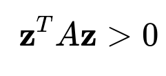
A positive definite matrix is a real, symmetric matrix that yields strictly positive values when used in a certain quadratic form with a non-zero vector. The classic condition is shown here:

This means that for any non-zero vector z, the expression z^T A z is strictly greater than 0, reflecting the fact that A is positive definite. Such a matrix is also invertible. Transforming a vector z by a positive definite matrix has geometric and algebraic interpretations.

Geometrically, the transformation preserves the general orientation of vectors but may stretch or contract them. Positive definiteness guarantees that no direction collapses entirely to zero, so lengths are scaled in a way that never becomes degenerate. The transformation often manifests as an elliptical stretching if we visualize how the unit sphere is mapped under A.

Algebraically, applying A to z results in a new vector A z. The fact that the matrix is positive definite guarantees that the quadratic form on z has a positive value for all non-zero z. From an eigen-decomposition standpoint, a positive definite matrix can be expressed as Q Lambda Q^T in text-based form, where Lambda has strictly positive eigenvalues. This leads to a transformation that remains invertible, with each direction scaled by the positive eigenvalues.

In practical scenarios such as optimization problems, a positive definite matrix is frequently seen as the Hessian of a strictly convex function, ensuring there is a unique global minimum. Similarly, in multivariate statistics, the covariance matrix must be positive definite (or at least positive semi-definite) to ensure valid variance estimates.

Implementation-wise, one can check for positive definiteness by performing a Cholesky decomposition or examining eigenvalues. Cholesky decomposition requires that the matrix be symmetric and that all leading principal minors be positive. If any condition fails, the matrix is not positive definite. When applying such a matrix to a vector, it is guaranteed that the result is an invertible linear mapping that can be reversed by the inverse of A.

Follow-up Question: How can one verify if a matrix is positive definite in practical code?

One common approach is the Cholesky decomposition, which fails if the matrix is not positive definite. Another method is to check that all eigenvalues are strictly greater than zero. Here is a Python snippet illustrating one approach:

import numpy as np

def is_positive_definite(A):
    # Method 1: Try Cholesky factorization
    try:
        np.linalg.cholesky(A)
        return True
    except np.linalg.LinAlgError:
        return False

# Example usage
matrix = np.array([[2, 1],
                   [1, 2]], dtype=float)

print(is_positive_definite(matrix))  # Expected True for this example

If the decomposition succeeds, the matrix is positive definite; otherwise, a numerical error is raised. Alternatively, one can compute all the eigenvalues and check if each is greater than zero. Matrices arising in data science contexts (such as covariance matrices) should theoretically be positive semi-definite, but numerical imprecision can lead to near-zero or small negative eigenvalues, so robust checks are important.

Follow-up Question: How does a positive definite transform differ from an orthonormal transform?

A positive definite transform, in general, changes lengths of vectors in a way that depends on the matrix’s eigenvalues, which are strictly positive but not necessarily equal to 1. Hence, vectors can be scaled by different amounts in different directions.

An orthonormal transform, by contrast, preserves lengths of vectors completely because its matrix is orthogonal and its inverse is its transpose. The eigenvalues in that case are typically 1 or -1 (depending on whether it is purely orthogonal or includes reflections), so no scaling of lengths occurs.

Follow-up Question: Why does positive definiteness ensure that no vector is mapped to the zero vector other than the trivial zero vector?

Positive definiteness means z^T A z is strictly greater than zero for any non-zero z. If a non-zero vector were mapped to the zero vector, it would imply A z = 0 for that vector. This would produce z^T A z = z^T 0 = 0, which contradicts the requirement that z^T A z > 0 for all non-zero z. Hence, the transformation can never collapse a non-zero vector to the zero vector, implying invertibility.

Follow-up Question: How does this property help in optimization?

When A represents the Hessian of a function in an optimization problem, positive definiteness ensures that the function is strictly convex. A strictly convex function has a single global minimum and no local minima distinct from the global one. During gradient-based optimization, the presence of a positive definite Hessian allows methods like Newton’s method to converge more reliably and swiftly to a unique optimum.

Follow-up Question: What are possible pitfalls when dealing with large matrices in practical scenarios?

In large-dimensional problems, numerical stability is a concern. Rounding errors might cause a matrix that is theoretically positive definite to appear slightly indefinite, resulting in failed factorizations or negative eigenvalues that should not be negative. Preconditioning, regularization, or adding small diagonal values (jitter) can address numerical issues. Data with near-collinearity can also produce covariance matrices that have very small eigenvalues, leading to numerical problems when attempting to invert the matrix.

In code, setting tolerances or using robust decomposition methods can mitigate these risks. Additionally, verifying the matrix’s condition number can help assess whether the transform might produce excessive numerical errors.